4.6: Runge-Kutta methods

The most famous predictor-corrector methods are the Runge-Kutta methods. Even if you have had only passing familiarity with numerical methods for ODEs in the past, you have probably heard of these methods, or even used them! In particular, 4th-order Runge-Kutta is the most common workhorse used when solving ODEs. It is the go-to solver used to solve the majority of ODEs. A variant of 4th-order Runge-Kutta is built into Matlab as the function ode45. There are plenty of other ODE solvers available, but one generally tries 4th order Runge-Kutta first, and if it doesn’t work or produces poor results then one turns to other, more specialized methods.

We will concentrate on the classic 4th order Runge-Kutta method since it is the most common one. Runge-Kutta methods of other orders also exist, but this 4th order method is both most common and also shows all the relevant concepts you should learn. In any event, you will likely call a pre-written solver from a library in your real work, so the important thing to learn are the concepts involved, not the details of each and every variant in the Runge-Kutta family.

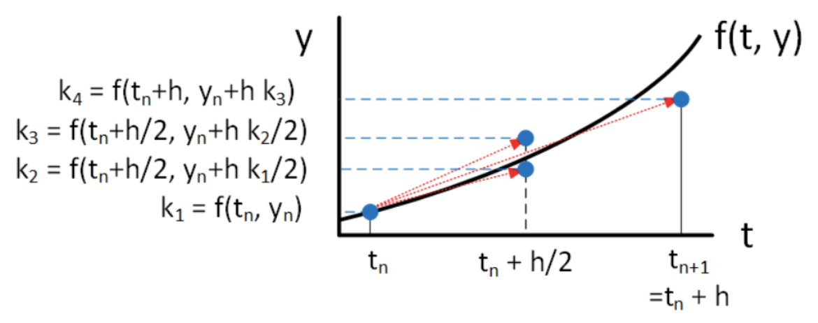
In what follows we will call this particular variant of 4th order Runge Kutta "RK4" for brevity. RK4 takes four samples of the present and future slopes. Here is the method:

\[\begin{aligned} \nonumber k_1 &= h f(t_n, y_n) \\ \nonumber k_2 &= h f(t_n+h/2, y_n + k_1/2) \\ \nonumber k_3 &= h f(t_n+h/2, y_n + k_2/2) \\ \nonumber k_4 &= h f(t_n+h, y_n + k_3) \\ \nonumber y_{n+1} &= y_n + (k_1 + 2 k_2 + 2 k_3 + k_4)/6\end{aligned}\]

Things to note about RK4:

• RK4 computes four intermediate results, \(k_1\), \(k_2\), \(k_3\), \(k_4\). Each intermediate result relies on the preceeding computation – that means you must perform the computations in order. The computation is depicted graphically in 4.9.
• The final result is a weighted sum of the intermediate results.
• RK4 is an explicit method – no rootfinding is required to compute the desired result.
• You might wonder where the sample points and the coefficients in the weighted sum come from. The short answer is, they are something you look up in a book (or online). The longer answer is, of course they may be derived, but the derivation is long and tedious and doesn’t lend any insight into the method. Therefore, we will skip the derivation here.
• We have depicted \(y\) to be a scalar in the above – that is, we assumed we are solving a single, scalar ODE. However, just as in the previous methods, \(y\) may also be a vector – that is, RK4 may also be used to solve a system of ODEs in the same way as may be used for all previous methods.

Figure 4.9: Fourth order Runge-Kutta intermediate results depicted graphically. The method relies on sampling the slope of the function \(f(t, y)\) at four different locations in order to compute the final step. The sample locations are built up sequentially. Note that two of the locations lie one-half way between the current time \(t_n\) and the final time \(t_{n+1}\).