Mathematics LibreTexts

13.5: Conformal interpretation

  • Page ID
    23665
  • \( \newcommand{\vecs}[1]{\overset { \scriptstyle \rightharpoonup} {\mathbf{#1}} } \)

    \( \newcommand{\vecd}[1]{\overset{-\!-\!\rightharpoonup}{\vphantom{a}\smash {#1}}} \)

    \( \newcommand{\id}{\mathrm{id}}\) \( \newcommand{\Span}{\mathrm{span}}\)

    ( \newcommand{\kernel}{\mathrm{null}\,}\) \( \newcommand{\range}{\mathrm{range}\,}\)

    \( \newcommand{\RealPart}{\mathrm{Re}}\) \( \newcommand{\ImaginaryPart}{\mathrm{Im}}\)

    \( \newcommand{\Argument}{\mathrm{Arg}}\) \( \newcommand{\norm}[1]{\| #1 \|}\)

    \( \newcommand{\inner}[2]{\langle #1, #2 \rangle}\)

    \( \newcommand{\Span}{\mathrm{span}}\)

    \( \newcommand{\id}{\mathrm{id}}\)

    \( \newcommand{\Span}{\mathrm{span}}\)

    \( \newcommand{\kernel}{\mathrm{null}\,}\)

    \( \newcommand{\range}{\mathrm{range}\,}\)

    \( \newcommand{\RealPart}{\mathrm{Re}}\)

    \( \newcommand{\ImaginaryPart}{\mathrm{Im}}\)

    \( \newcommand{\Argument}{\mathrm{Arg}}\)

    \( \newcommand{\norm}[1]{\| #1 \|}\)

    \( \newcommand{\inner}[2]{\langle #1, #2 \rangle}\)

    \( \newcommand{\Span}{\mathrm{span}}\) \( \newcommand{\AA}{\unicode[.8,0]{x212B}}\)

    \( \newcommand{\vectorA}[1]{\vec{#1}}      % arrow\)

    \( \newcommand{\vectorAt}[1]{\vec{\text{#1}}}      % arrow\)

    \( \newcommand{\vectorB}[1]{\overset { \scriptstyle \rightharpoonup} {\mathbf{#1}} } \)

    \( \newcommand{\vectorC}[1]{\textbf{#1}} \)

    \( \newcommand{\vectorD}[1]{\overrightarrow{#1}} \)

    \( \newcommand{\vectorDt}[1]{\overrightarrow{\text{#1}}} \)

    \( \newcommand{\vectE}[1]{\overset{-\!-\!\rightharpoonup}{\vphantom{a}\smash{\mathbf {#1}}}} \)

    \( \newcommand{\vecs}[1]{\overset { \scriptstyle \rightharpoonup} {\mathbf{#1}} } \)

    \( \newcommand{\vecd}[1]{\overset{-\!-\!\rightharpoonup}{\vphantom{a}\smash {#1}}} \)

    \(\newcommand{\avec}{\mathbf a}\) \(\newcommand{\bvec}{\mathbf b}\) \(\newcommand{\cvec}{\mathbf c}\) \(\newcommand{\dvec}{\mathbf d}\) \(\newcommand{\dtil}{\widetilde{\mathbf d}}\) \(\newcommand{\evec}{\mathbf e}\) \(\newcommand{\fvec}{\mathbf f}\) \(\newcommand{\nvec}{\mathbf n}\) \(\newcommand{\pvec}{\mathbf p}\) \(\newcommand{\qvec}{\mathbf q}\) \(\newcommand{\svec}{\mathbf s}\) \(\newcommand{\tvec}{\mathbf t}\) \(\newcommand{\uvec}{\mathbf u}\) \(\newcommand{\vvec}{\mathbf v}\) \(\newcommand{\wvec}{\mathbf w}\) \(\newcommand{\xvec}{\mathbf x}\) \(\newcommand{\yvec}{\mathbf y}\) \(\newcommand{\zvec}{\mathbf z}\) \(\newcommand{\rvec}{\mathbf r}\) \(\newcommand{\mvec}{\mathbf m}\) \(\newcommand{\zerovec}{\mathbf 0}\) \(\newcommand{\onevec}{\mathbf 1}\) \(\newcommand{\real}{\mathbb R}\) \(\newcommand{\twovec}[2]{\left[\begin{array}{r}#1 \\ #2 \end{array}\right]}\) \(\newcommand{\ctwovec}[2]{\left[\begin{array}{c}#1 \\ #2 \end{array}\right]}\) \(\newcommand{\threevec}[3]{\left[\begin{array}{r}#1 \\ #2 \\ #3 \end{array}\right]}\) \(\newcommand{\cthreevec}[3]{\left[\begin{array}{c}#1 \\ #2 \\ #3 \end{array}\right]}\) \(\newcommand{\fourvec}[4]{\left[\begin{array}{r}#1 \\ #2 \\ #3 \\ #4 \end{array}\right]}\) \(\newcommand{\cfourvec}[4]{\left[\begin{array}{c}#1 \\ #2 \\ #3 \\ #4 \end{array}\right]}\) \(\newcommand{\fivevec}[5]{\left[\begin{array}{r}#1 \\ #2 \\ #3 \\ #4 \\ #5 \\ \end{array}\right]}\) \(\newcommand{\cfivevec}[5]{\left[\begin{array}{c}#1 \\ #2 \\ #3 \\ #4 \\ #5 \\ \end{array}\right]}\) \(\newcommand{\mattwo}[4]{\left[\begin{array}{rr}#1 \amp #2 \\ #3 \amp #4 \\ \end{array}\right]}\) \(\newcommand{\laspan}[1]{\text{Span}\{#1\}}\) \(\newcommand{\bcal}{\cal B}\) \(\newcommand{\ccal}{\cal C}\) \(\newcommand{\scal}{\cal S}\) \(\newcommand{\wcal}{\cal W}\) \(\newcommand{\ecal}{\cal E}\) \(\newcommand{\coords}[2]{\left\{#1\right\}_{#2}}\) \(\newcommand{\gray}[1]{\color{gray}{#1}}\) \(\newcommand{\lgray}[1]{\color{lightgray}{#1}}\) \(\newcommand{\rank}{\operatorname{rank}}\) \(\newcommand{\row}{\text{Row}}\) \(\newcommand{\col}{\text{Col}}\) \(\renewcommand{\row}{\text{Row}}\) \(\newcommand{\nul}{\text{Nul}}\) \(\newcommand{\var}{\text{Var}}\) \(\newcommand{\corr}{\text{corr}}\) \(\newcommand{\len}[1]{\left|#1\right|}\) \(\newcommand{\bbar}{\overline{\bvec}}\) \(\newcommand{\bhat}{\widehat{\bvec}}\) \(\newcommand{\bperp}{\bvec^\perp}\) \(\newcommand{\xhat}{\widehat{\xvec}}\) \(\newcommand{\vhat}{\widehat{\vvec}}\) \(\newcommand{\uhat}{\widehat{\uvec}}\) \(\newcommand{\what}{\widehat{\wvec}}\) \(\newcommand{\Sighat}{\widehat{\Sigma}}\) \(\newcommand{\lt}{<}\) \(\newcommand{\gt}{>}\) \(\newcommand{\amp}{&}\) \(\definecolor{fillinmathshade}{gray}{0.9}\)

    Let us give another interpretation of the h-distance.

    Lemma \(\PageIndex{1}\)

    Consider the h-plane with the unit circle centered at \(O\) as the absolute. Fix a point \(P\) and let \(Q\) be another point in the h-plane. Set \(x = PQ\) and \(y = PQ_h\). Then

    \[\lim_{x\to 0} \dfrac{y}{x} = \dfrac{2}{1-OP^2}.\]

    The above formula tells us that the h-distance from \(P\) to a nearby point \(Q\) is almost proportional to the Euclidean distance with the coefficient \(\dfrac{2}{1-OP^2}\). The value \(\lambda(P)=\dfrac{2}{1-OP^2}\) is called the conformal factor of the h-metric.

    The value \(\dfrac{1}{\lambda(P)}=\dfrac{1}{2} \cdot (1-OP^2)\) can be interpreted as the speed limit at the given point \(P\). In this case the h-distance is the minimal time needed to travel from one point of the h-plane to another point.
    截屏2021-02-24 下午4.10.21.png

    Proof

    If \(P=O\), then according to Lemma 12.3.2

    \[\dfrac{y}{x}=\dfrac{\ln \dfrac{1+x}{1-x}}{x}\to 2\]

    as \(x\to0\).

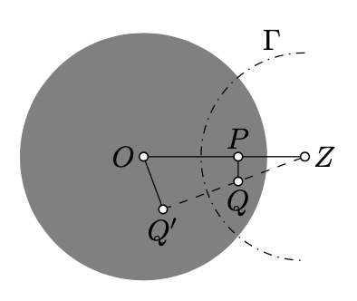
    If \(P\ne O\), let \(Z\) denotes the inverse of \(P\) in the absolute. Suppose that \(\Gamma\) denotes the circle with the center \(Z\) perpendicular to the absolute.

    According to the main observation (Theorem 12.3.1) and Lemma 12.3.1, the inversion in \(\Gamma\) is a motion of the h-plane which sends \(P\) to \(O\). In particular, if \(Q'\) denotes the inverse of \(Q\) in \(\Gamma\), then \(OQ'_h=PQ_h\).

    Set \(x'=OQ'\). According to Lemma 10.1.1,

    \(\dfrac{x'}{x}=\dfrac{OZ}{ZQ}.\)

    Since \(Z\) is the inverse of \(P\) in the absolute, we have that \(PO\cdot OZ=1\). Therefore,

    as \(x \to 0\).

    According to 13.5.1, \(\dfrac{y}{x'} \to 2\) as \(x' \to 0\). Therefore

    as \(x \to 0\).

    Here is an application of the lemma above.

    Proposition \(\PageIndex{1}\)

    The circumference of an h-circle of the h-radius \(r\) is

    \(2 \cdot \pi \cdot \sinh r,\)

    where \(\sinh r\) denotes the hyperbolic sine of \(r\); that is,

    \(\sinh r := \dfrac{e^r-e^{-r}}{2}.\)

    Before we proceed with the proof, let us discuss the same problem in the Euclidean plane.

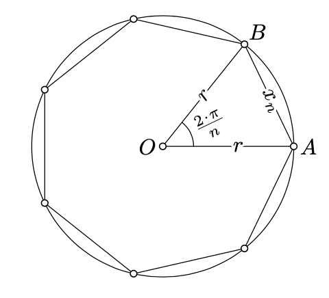
    The circumference of a circle in the Euclidean plane can be defined as the limit of perimeters of regular \(n\)-gons inscribed in the circle as \(n \to \infty\).

    Namely, let us fix \(r>0\). Given a positive integer \(n\), consider \(\triangle AOB\) such that \(\measuredangle AOB=\dfrac{2\cdot\pi}{n}\) and \(OA=OB=r\). Set \(x_n=AB\). Note that \(x_n\) is the side of a regular \(n\)-gon inscribed in the circle of radius \(r\). Therefore, the perimeter of the \(n\)-gon is \(n\cdot x_n\).
    截屏2021-02-25 上午8.50.40.png

    The circumference of the circle with the radius \(r\) might be defined as the limit

    \[\lim_{n\to\infty} n\cdot x_n=2\cdot\pi\cdot r.\]

    (This limit can be taken as the definition of \(\pi\).)

    In the following proof, we repeat the same construction in the h-plane.

    Proof

    Without loss of generality, we can assume that the center \(O\) of the circle is the center of the absolute.

    By Lemma 12.3.2, the h-circle with the h-radius \(r\) is the Euclidean circle with the center \(O\) and the radius

    \(a=\dfrac{e^r-1}{e^r+1}.\)

    Let \(x_n\) and \(y_n\) denote the side lengths of the regular \(n\)-gons inscribed in the circle in the Euclidean and hyperbolic plane respectively.

    Note that \(x_n\to0\) as \(n\to\infty\). By Lemma \(\PageIndecx{1}\),

    \(\lim_{n\to\infty} \dfrac{y_n}{x_n} = \dfrac{2}{1-a^2}.\)

    Applying 13.5.2, we get that the circumference of the h-circle can be found the following way:

    \(\begin{array} {rcl} {\lim_{n \to \infty} n \cdot y_n} & = & {\dfrac{2}{1 - a^2} \cdot \lim_{n \to \infty} n \cdot x_n =} \\ {} & = & {\dfrac{4 \cdot \pi \cdot a}{1 - a^2} =} \\ {} & = & {\dfrac{4 \cdot \pi \cdot (\dfrac{e^r - 1}{e^r + 1})}{1 - (\dfrac{e^r - 1}{e^r + 1})^2} =} \\ {} & = & {2 \cdot \pi \cdot \dfrac{e^r - e^{-r}}{2} =} \\ {} & = & {2 \cdot \pi \cdot \sinh r.} \end{array}\)

    Exercise \(\PageIndex{1}\)

    Let \(\circum_h(r)\) denote the circumference of the h-circle of the h-radius \(r\). Show that

    \(\\text{circum}_h(r+1)>2\cdot \text{circum}_h(r)\])

    for all \(r>0\).

    Hint

    Apply Proposition \(\PageIndex{1}\). Use that \(e > 2\) and in particular the function \(r \mapsto e^{-r}\) is decreasing.


    This page titled 13.5: Conformal interpretation is shared under a CC BY-SA 4.0 license and was authored, remixed, and/or curated by Anton Petrunin via source content that was edited to the style and standards of the LibreTexts platform.