
7.4: Orthogonality
- Page ID
- 14541

Orthogonal Diagonalization
We begin this section by recalling some important definitions. Recall from Definition 4.11.4 that non-zero vectors are called orthogonal if their dot product equals \(0\). A set is orthonormal if it is orthogonal and each vector is a unit vector.
An orthogonal matrix \(U\), from Definition 4.11.7, is one in which \(UU^{T} = I\). In other words, the transpose of an orthogonal matrix is equal to its inverse. A key characteristic of orthogonal matrices, which will be essential in this section, is that the columns of an orthogonal matrix form an orthonormal set.
We now recall another important definition.
A real \(n\times n\) matrix \(A,\) is symmetric if \(A^{T}=A.\) If \( A=-A^{T},\) then \(A\) is called skew symmetric.
Before proving an essential theorem, we first examine the following lemma which will be used below.
Let \(A=\left ( a_{ij} \right )\) be a real symmetric \(n \times n\) matrix, and let \(\vec{x}, \vec{y} \in \mathbb{R}^n\). Then \[A\vec{x} \cdot \vec{y} = \vec{x} \cdot A \vec{y}\nonumber\]
- Proof
-
This result follows from the definition of the dot product together with properties of matrix multiplication, as follows: \[\begin{aligned} A\vec{x} \cdot \vec{y} &= \sum_{k,l}a_{kl}x_{l}y_{k} \\ &=\sum_{k,l} (a_{lk})^Tx_{l}y_{k} \\ &= \vec{x}\cdot A^{T}\vec{y} \\ &= \vec{x}\cdot A \vec{y}\end{aligned}\]
The last step follows from \(A^T = A\), since \(A\) is symmetric.
We can now prove that the eigenvalues of a real symmetric matrix are real numbers. Consider the following important theorem.
Let \(A\) be a real symmetric matrix. Then the eigenvalues of \(A\) are real numbers and eigenvectors corresponding to distinct eigenvalues are orthogonal.
- Proof
-
Recall that for a complex number \(a+ib,\) the complex conjugate, denoted by \(\overline{a+ib}\) is given by \(\overline{a+ib}=a-ib.\) The notation, \(\overline{\vec{x}}\) will denote the vector which has every entry replaced by its complex conjugate.
Suppose \(A\) is a real symmetric matrix and \(A\vec{x}=\lambda \vec{x}\). Then \[\overline{\lambda \vec{x}}^{T}\vec{x}=\left( \overline{A \vec{x}}\right) ^{T}\vec{x}=\overline{\vec{x}}^{T}A^{T}\vec{x}= \overline{\vec{x}}^{T}A\vec{x}=\lambda \overline{\vec{x}}^{T} \vec{x}\nonumber \] Dividing by \(\overline{\vec{x}}^{T}\vec{x}\) on both sides yields \(\overline{\lambda }=\lambda\) which says \(\lambda\) is real. To do this, we need to ensure that \(\overline{\vec{x}}^{T}\vec{x} \neq 0\). Notice that \(\overline{\vec{x}}^{T}\vec{x} = 0\) if and only if \(\vec{x} = \vec{0}\). Since we chose \(\vec{x}\) such that \(A\vec{x} = \lambda \vec{x}\), \(\vec{x}\) is an eigenvector and therefore must be nonzero.
Now suppose \(A\) is real symmetric and \(A\vec{x}=\lambda \vec{x}\), \(A \vec{y}=\mu \vec{y}\) where \(\mu \neq \lambda\). Then since \(A\) is symmetric, it follows from Lemma \(\PageIndex{1}\) about the dot product that \[\lambda \vec{x}\cdot \vec{y}=A\vec{x}\cdot \vec{y}=\vec{x}\cdot A\vec{y}=\vec{x}\cdot \mu \vec{y}=\mu \vec{x}\cdot \vec{y}\nonumber \] Hence \(\left( \lambda -\mu \right) \vec{x}\cdot \vec{y}=0.\) It follows that, since \(\lambda -\mu \neq 0,\) it must be that \(\vec{x}\cdot \vec{y}=0\). Therefore the eigenvectors form an orthogonal set.
The following theorem is proved in a similar manner.
The eigenvalues of a real skew symmetric matrix are either equal to \(0\) or are pure imaginary numbers.
- Proof
-
First, note that if \(A=0\) is the zero matrix, then \(A\) is skew symmetric and has eigenvalues equal to \(0\).
Suppose \(A=-A^{T}\) so \(A\) is skew symmetric and \(A\vec{x}=\lambda \vec{x}\). Then \[\overline{\lambda \vec{x}}^{T}\vec{x}=\left( \overline{A \vec{x}}\right) ^{T}\vec{x}=\overline{\vec{x}}^{T}A^{T}\vec{x}=- \overline{\vec{x}}^{T}A\vec{x}=-\lambda \overline{\vec{x}}^{T} \vec{x}\nonumber \] and so, dividing by \(\overline{\vec{x}}^{T}\vec{x}\) as before, \(\overline{\lambda }=-\lambda .\) Letting \(\lambda =a+ib,\) this means \(a-ib=-a-ib\) and so \(a=0.\) Thus \(\lambda\) is pure imaginary.
Consider the following example.
Let \(A=\left[ \begin{array}{rr} 0 & -1 \\ 1 & 0 \end{array} \right] .\) Find its eigenvalues.
Solution
First notice that \(A\) is skew symmetric. By Theorem \(\PageIndex{2}\), the eigenvalues will either equal \(0\) or be pure imaginary. The eigenvalues of \(A\) are obtained by solving the usual equation \[\det (\lambda I - A ) = \det \left[ \begin{array}{rr} \lambda & 1 \\ -1 & \lambda \end{array} \right] =\lambda ^{2}+1=0\nonumber \]
Hence the eigenvalues are \(\pm i,\) pure imaginary.
Consider the following example.
Let \(A=\left[ \begin{array}{rr} 1 & 2 \\ 2 & 3 \end{array} \right] .\) Find its eigenvalues.
Solution
First, notice that \(A\) is symmetric. By Theorem \(\PageIndex{1}\), the eigenvalues will all be real. The eigenvalues of \(A\) are obtained by solving the usual equation \[\det (\lambda I - A) = \det \left[ \begin{array}{rr} \lambda - 1 & -2 \\ -2 & \lambda - 3 \end{array} \right] = \lambda^2 -4\lambda -1=0\nonumber \] The eigenvalues are given by \(\lambda_1 =2+ \sqrt{5}\) and \(\lambda_2 =2-\sqrt{5}\) which are both real.
Recall that a diagonal matrix \(D=\left ( d_{ij} \right )\) is one in which \(d_{ij} = 0\) whenever \(i \neq j\). In other words, all numbers not on the main diagonal are equal to zero.
Consider the following important theorem.
Let \(A\) be a real symmetric matrix. Then there exists an orthogonal matrix \(U\) such that \[U^{T}AU = D\nonumber \] where \(D\) is a diagonal matrix. Moreover, the diagonal entries of \(D\) are the eigenvalues of \(A\).
We can use this theorem to diagonalize a symmetric matrix, using orthogonal matrices. Consider the following corollary.
If \(A\) is a real \(n\times n\) symmetric matrix, then there exists an orthonormal set of eigenvectors, \(\left\{ \vec{u}_{1},\cdots ,\vec{u} _{n}\right\} .\)
- Proof
-
Since \(A\) is symmetric, then by Theorem \(\PageIndex{3}\), there exists an orthogonal matrix \(U\) such that \(U^{T}AU=D,\) a diagonal matrix whose diagonal entries are the eigenvalues of \(A.\) Therefore, since \(A\) is symmetric and all the matrices are real, \[\overline{D}=\overline{D^{T}}=\overline{U^{T}A^{T}U}=U^{T}A^{T}U=U^{T}AU=D\nonumber \] showing \(D\) is real because each entry of \(D\) equals its complex conjugate.
Now let \[U=\left[ \begin{array}{cccc} \vec{u}_{1} & \vec{u}_{2} & \cdots & \vec{u}_{n} \end{array} \right]\nonumber \] where the \(\vec{u}_{i}\) denote the columns of \(U\) and \[D=\left[ \begin{array}{ccc} \lambda _{1} & & 0 \\ & \ddots & \\ 0 & & \lambda _{n} \end{array} \right]\nonumber \] The equation, \(U^{T}AU=D\) implies \(AU = UD\) and \[\begin{aligned} AU &=\left[ \begin{array}{cccc} A\vec{u}_{1} & A\vec{u}_{2} & \cdots & A\vec{u}_{n} \end{array} \right] \\ &=\left[ \begin{array}{cccc} \lambda _{1}\vec{u}_{1} & \lambda _{2}\vec{u}_{2} & \cdots & \lambda _{n}\vec{u}_{n} \end{array} \right] \\ &= UD\end{aligned}\] where the entries denote the columns of \(AU\) and \(UD\) respectively. Therefore, \(A\vec{u}_{i}=\lambda _{i}\vec{u}_{i}\). Since the matrix \(U\) is orthogonal, the \(ij^{th}\) entry of \(U^{T}U\) equals \(\delta _{ij}\) and so \[\delta _{ij}=\vec{u}_{i}^{T}\vec{u}_{j}=\vec{u}_{i}\cdot \vec{u} _{j}\nonumber \] This proves the corollary because it shows the vectors \(\left\{ \vec{u} _{i}\right\}\) form an orthonormal set.
Let \(A\) be an \(n \times n\) matrix. Then the principal axes of \(A\) is a set of orthonormal eigenvectors of \(A\).
In the next example, we examine how to find such a set of orthonormal eigenvectors.
Find an orthonormal set of eigenvectors for the symmetric matrix \[A = \left[ \begin{array}{rrr} 17 & -2 & -2 \\ -2 & 6 & 4 \\ -2 & 4 & 6 \end{array} \right]\nonumber \]
Solution
Recall Procedure 7.1.1 for finding the eigenvalues and eigenvectors of a matrix. You can verify that the eigenvalues are \(18,9,2.\) First find the eigenvector for \(18\) by solving the equation \((18I-A)X = 0\). The appropriate augmented matrix is given by \[\left[ \begin{array}{ccc|c} 18-17 & 2 & 2 & 0 \\ 2 & 18-6 & -4 & 0 \\ 2 & -4 & 18-6 & 0 \end{array} \right]\nonumber \] The reduced row-echelon form is \[\left[ \begin{array}{rrr|r} 1 & 0 & 4 & 0 \\ 0 & 1 & -1 & 0 \\ 0 & 0 & 0 & 0 \end{array} \right]\nonumber \] Therefore an eigenvector is \[\left[ \begin{array}{r} -4 \\ 1 \\ 1 \end{array} \right]\nonumber \] Next find the eigenvector for \(\lambda =9.\) The augmented matrix and resulting reduced row-echelon form are \[\left[ \begin{array}{ccc|c} 9-17 & 2 & 2 & 0 \\ 2 & 9-6 & -4 & 0 \\ 2 & -4 & 9-6 & 0 \end{array} \right] \rightarrow \cdots \rightarrow \left[ \begin{array}{rrr|r} 1 & 0 & - \frac{1}{2} & 0 \\ 0 & 1 & -1 & 0 \\ 0 & 0 & 0 & 0 \end{array} \right]\nonumber \] Thus an eigenvector for \(\lambda =9\) is \[\left[ \begin{array}{r} 1 \\ 2 \\ 2 \end{array} \right]\nonumber \] Finally find an eigenvector for \(\lambda =2.\) The appropriate augmented matrix and reduced row-echelon form are \[\left[ \begin{array}{ccc|c} 2-17 & 2 & 2 & 0 \\ 2 & 2-6 & -4 & 0 \\ 2 & -4 & 2-6 & 0 \end{array} \right] \rightarrow \cdots \rightarrow \left[ \begin{array}{rrr|r} 1 & 0 & 0 & 0 \\ 0 & 1 & 1 & 0 \\ 0 & 0 & 0 & 0 \end{array} \right]\nonumber \] Thus an eigenvector for \(\lambda =2\) is \[\left[ \begin{array}{r} 0 \\ -1 \\ 1 \end{array} \right]\nonumber \]
The set of eigenvectors for \(A\) is given by \[\left\{ \left[ \begin{array}{r} -4 \\ 1 \\ 1 \end{array} \right], \left[ \begin{array}{r} 1 \\ 2 \\ 2 \end{array} \right], \left[ \begin{array}{r} 0 \\ -1 \\ 1 \end{array} \right] \right\}\nonumber \] You can verify that these eigenvectors form an orthogonal set. By dividing each eigenvector by its magnitude, we obtain an orthonormal set: \[\left\{ \frac{1}{\sqrt{18}}\left[ \begin{array}{r} -4 \\ 1 \\ 1 \end{array} \right] ,\frac{1}{3}\left[ \begin{array}{r} 1 \\ 2 \\ 2 \end{array} \right] ,\frac{1}{\sqrt{2}}\left[ \begin{array}{r} 0 \\ -1 \\ 1 \end{array} \right] \right\}\nonumber \]
Consider the following example.
Find an orthonormal set of three eigenvectors for the matrix \[A = \left[ \begin{array}{rrr} 10 & 2 & 2 \\ 2 & 13 & 4 \\ 2 & 4 & 13 \end{array} \right]\nonumber \]
Solution
You can verify that the eigenvalues of \(A\) are \(9\) (with multiplicity two) and \(18\) (with multiplicity one). Consider the eigenvectors corresponding to \(\lambda =9\). The appropriate augmented matrix and reduced row-echelon form are given by \[\left[ \begin{array}{ccc|c} 9-10 & -2 & -2 & 0 \\ -2 & 9-13 & -4 & 0 \\ -2 & -4 & 9-13 & 0 \end{array} \right] \rightarrow \cdots \rightarrow \left[ \begin{array}{rrr|r} 1 & 2 & 2 & 0 \\ 0 & 0 & 0 & 0 \\ 0 & 0 & 0 & 0 \end{array} \right]\nonumber \] and so eigenvectors are of the form \[\left[ \begin{array}{c} -2y-2z \\ y \\ z \end{array} \right]\nonumber \] We need to find two of these which are orthogonal. Let one be given by setting \(z=0\) and \(y=1\), giving \(\left[ \begin{array}{r} -2 \\ 1 \\ 0 \end{array} \right]\).
In order to find an eigenvector orthogonal to this one, we need to satisfy \[\left[ \begin{array}{r} -2 \\ 1 \\ 0 \end{array} \right] \cdot \left[ \begin{array}{c} -2y-2z \\ y \\ z \end{array} \right] =5y+4z=0\nonumber \] The values \(y=-4\) and \(z=5\) satisfy this equation, giving another eigenvector corresponding to \(\lambda=9\) as \[\left[ \begin{array}{c} -2\left( -4\right) -2\left( 5\right) \\ \left( -4\right) \\ 5 \end{array} \right] =\left[ \begin{array}{r} -2 \\ -4 \\ 5 \end{array} \right]\nonumber \] Next find the eigenvector for \(\lambda =18.\) The augmented matrix and the resulting reduced row-echelon form are given by \[\left[ \begin{array}{ccc|c} 18-10 & -2 & -2 & 0 \\ -2 & 18-13 & -4 & 0 \\ -2 & -4 & 18-13 & 0 \end{array} \right] \rightarrow \cdots \rightarrow \left[ \begin{array}{rrr|r} 1 & 0 & - \frac{1}{2} & 0 \\ 0 & 1 & -1 & 0 \\ 0 & 0 & 0 & 0 \end{array} \right]\nonumber \] and so an eigenvector is \[\left[ \begin{array}{r} 1 \\ 2 \\ 2 \end{array} \right]\nonumber \]
Dividing each eigenvector by its length, the orthonormal set is \[\left\{ \frac{1}{\sqrt{5}} \left[ \begin{array}{r} -2\\ 1 \\ 0 \end{array} \right] , \frac{\sqrt{5}}{15} \left[ \begin{array}{r} -2 \\ -4 \\ 5 \end{array} \right] , \frac{1}{3}\left[ \begin{array}{r} 1 \\ 2 \\ 2 \end{array} \right] \right\}\nonumber \]
In the above solution, the repeated eigenvalue implies that there would have been many other orthonormal bases which could have been obtained. While we chose to take \(z=0, y=1\), we could just as easily have taken \(y=0\) or even \(y=z=1.\) Any such change would have resulted in a different orthonormal set.
Recall the following definition.
An \(n\times n\) matrix \(A\) is said to be non defective or diagonalizable if there exists an invertible matrix \(P\) such that \(P^{-1}AP=D\) where \(D\) is a diagonal matrix.
As indicated in Theorem \(\PageIndex{3}\) if \(A\) is a real symmetric matrix, there exists an orthogonal matrix \(U\) such that \(U^{T}AU=D\) where \(D\) is a diagonal matrix. Therefore, every symmetric matrix is diagonalizable because if \(U\) is an orthogonal matrix, it is invertible and its inverse is \(U^{T}\). In this case, we say that \(A\) is orthogonally diagonalizable. Therefore every symmetric matrix is in fact orthogonally diagonalizable. The next theorem provides another way to determine if a matrix is orthogonally diagonalizable.
Let \(A\) be an \(n \times n\) matrix. Then \(A\) is orthogonally diagonalizable if and only if \(A\) has an orthonormal set of eigenvectors.
Recall from Corollary \(\PageIndex{1}\) that every symmetric matrix has an orthonormal set of eigenvectors. In fact these three conditions are equivalent.
In the following example, the orthogonal matrix \(U\) will be found to orthogonally diagonalize a matrix.
Let \(A=\left[ \begin{array}{rrr} 1 & 0 & 0 \\ 0 & \frac{3}{2} & \frac{1}{2} \\ 0 & \frac{1}{2} & \frac{3}{2} \end{array} \right] .\) Find an orthogonal matrix \(U\) such that \(U^{T}AU\) is a diagonal matrix.
Solution
In this case, the eigenvalues are \(2\) (with multiplicity one) and \(1\) (with multiplicity two). First we will find an eigenvector for the eigenvalue \(2\). The appropriate augmented matrix and resulting reduced row-echelon form are given by \[\left[ \begin{array}{ccc|c} 2-1 & 0 & 0 & 0 \\ 0 & 2- \frac{3}{2} & - \frac{1}{2} & 0 \\ 0 & - \frac{1}{2} & 2- \frac{3}{2} & 0 \end{array} \right] \rightarrow \cdots \rightarrow \left[ \begin{array}{rrr|r} 1 & 0 & 0 & 0 \\ 0 & 1 & -1 & 0 \\ 0 & 0 & 0 & 0 \end{array} \right]\nonumber \] and so an eigenvector is \[\left[ \begin{array}{r} 0 \\ 1 \\ 1 \end{array} \right]\nonumber \] However, it is desired that the eigenvectors be unit vectors and so dividing this vector by its length gives \[\left[ \begin{array}{c} 0 \\ \frac{1}{\sqrt{2}} \\ \frac{1}{\sqrt{2}} \end{array} \right]\nonumber \] Next find the eigenvectors corresponding to the eigenvalue equal to \(1\). The appropriate augmented matrix and resulting reduced row-echelon form are given by: \[\left[ \begin{array}{ccc|c} 1-1 & 0 & 0 & 0 \\ 0 & 1- \frac{3}{2} & - \frac{1}{2} & 0 \\ 0 & - \frac{1}{2} & 1- \frac{3}{2} & 0 \end{array} \right] \rightarrow \cdots \rightarrow \left[ \begin{array}{rrr|r} 0 & 1 & 1 & 0 \\ 0 & 0 & 0 & 0 \\ 0 & 0 & 0 & 0 \end{array} \right]\nonumber \] Therefore, the eigenvectors are of the form \[\left[ \begin{array}{r} s \\ -t \\ t \end{array} \right]\nonumber \] Two of these which are orthonormal are \(\left[ \begin{array}{c} 1 \\ 0 \\ 0 \end{array} \right]\), choosing \(s=1\) and \(t=0\), and \(\left[ \begin{array}{c} 0 \\ - \frac{1}{\sqrt{2}} \\ \frac{1}{\sqrt{2}} \end{array} \right]\), letting \(s=0\), \(t= 1\) and normalizing the resulting vector.
To obtain the desired orthogonal matrix, we let the orthonormal eigenvectors computed above be the columns. \[\left[ \begin{array}{rrr} 0 & 1 & 0 \\ -\frac{1}{\sqrt{2}} & 0 & \frac{1}{\sqrt{2}} \\ \frac{1}{\sqrt{2}} & 0 & \frac{1}{\sqrt{2}} \end{array} \right]\nonumber \]
To verify, compute \(U^{T}AU\) as follows: \[U^{T}AU = \left[ \begin{array}{rrr} 0 & - \frac{1}{\sqrt{2}} & \frac{1}{\sqrt{2}} \\ 1 & 0 & 0 \\ 0 & \frac{1}{\sqrt{2}} & \frac{1}{\sqrt{2}} \end{array} \right] \left[ \begin{array}{rrr} 1 & 0 & 0 \\ 0 & \frac{3}{2} & \frac{1}{2} \\ 0 & \frac{1}{2} & \frac{3}{2} \end{array} \right] \left[ \begin{array}{rrr} 0 & 1 & 0 \\ -\frac{1}{\sqrt{2}} & 0 & \frac{1}{\sqrt{2}} \\ \frac{1}{\sqrt{2}} & 0 & \frac{1}{\sqrt{2}} \end{array} \right]\nonumber \] \[=\left[ \begin{array}{rrr} 1 & 0 & 0 \\ 0 & 1 & 0 \\ 0 & 0 & 2 \end{array} \right] = D\nonumber \] the desired diagonal matrix. Notice that the eigenvectors, which construct the columns of \(U\), are in the same order as the eigenvalues in \(D\).
We conclude this section with a Theorem that generalizes earlier results.
Let \(A\) be an \(n \times n\) matrix. If \(A\) has \(n\) real eigenvalues, then an orthogonal matrix \(U\) can be found to result in the upper triangular matrix \(U^T A U\).
triangulation
This Theorem provides a useful Corollary.
Let \(A\) be an \(n \times n\) matrix with eigenvalues \(\lambda_1, \cdots, \lambda_n\). Then it follows that \(\det(A)\) is equal to the product of the \(\lambda_i\), while \(trace(A)\) is equal to the sum of the \(\lambda_i\).
- Proof
-
By Theorem \(\PageIndex{5}\), there exists an orthogonal matrix \(U\) such that \(U^TAU=P\), where \(P\) is an upper triangular matrix. Since \(P\) is similar to \(A\), the eigenvalues of \(P\) are \(\lambda_1, \lambda_2, \ldots, \lambda_n\). Furthermore, since \(P\) is (upper) triangular, the entries on the main diagonal of \(P\) are its eigenvalues, so \(\det(P)=\lambda_1 \lambda_2 \cdots \lambda_n\) and \(trace(P)=\lambda_1 + \lambda_2 + \cdots + \lambda_n\). Since \(P\) and \(A\) are similar, \(\det(A)=\det(P)\) and \(trace(A)=trace(P)\), and therefore the results follow.
The Singular Value Decomposition
We begin this section with an important definition.
Let \(A\) be an \(m\times n\) matrix. The singular values of \(A\) are the square roots of the positive eigenvalues of \(A^TA.\)
Singular Value Decomposition (SVD) can be thought of as a generalization of orthogonal diagonalization of a symmetric matrix to an arbitrary \(m\times n\) matrix. This decomposition is the focus of this section.
The following is a useful result that will help when computing the SVD of matrices.
Let \(A\) be an \(m \times n\) matrix. Then \(A^TA\) and \(AA^T\) have the same nonzero eigenvalues.
- Proof
-
Suppose \(A\) is an \(m\times n\) matrix, and suppose that \(\lambda\) is a nonzero eigenvalue of \(A^TA\). Then there exists a nonzero vector \(X\in \mathbb{R}^n\) such that \[\label{nonzero} (A^TA)X=\lambda X.\]
Multiplying both sides of this equation by \(A\) yields: \[\begin{aligned} A(A^TA)X & = A\lambda X\\ (AA^T)(AX) & = \lambda (AX).\end{aligned}\] Since \(\lambda\neq 0\) and \(X\neq 0_n\), \(\lambda X\neq 0_n\), and thus by equation \(\eqref{nonzero}\), \((A^TA)X\neq 0_m\); thus \(A^T(AX)\neq 0_m\), implying that \(AX\neq 0_m\).
Therefore \(AX\) is an eigenvector of \(AA^T\) corresponding to eigenvalue \(\lambda\). An analogous argument can be used to show that every nonzero eigenvalue of \(AA^T\) is an eigenvalue of \(A^TA\), thus completing the proof.
Given an \(m\times n\) matrix \(A\), we will see how to express \(A\) as a product \[A=U\Sigma V^T\nonumber \] where
- \(U\) is an \(m\times m\) orthogonal matrix whose columns are eigenvectors of \(AA^T\).
- \(V\) is an \(n\times n\) orthogonal matrix whose columns are eigenvectors of \(A^TA\).
- \(\Sigma\) is an \(m\times n\) matrix whose only nonzero values lie on its main diagonal, and are the singular values of \(A\).
How can we find such a decomposition? We are aiming to decompose \(A\) in the following form:
\[A=U\left[ \begin{array}{cc} \sigma & 0 \\ 0 & 0 \end{array} \right] V^T\nonumber \] where \(\sigma\) is of the form \[\sigma =\left[ \begin{array}{ccc} \sigma _{1} & & 0 \\ & \ddots & \\ 0 & & \sigma _{k} \end{array} \right]\nonumber \]
Thus \(A^T=V\left[ \begin{array}{cc} \sigma & 0 \\ 0 & 0 \end{array} \right] U^T\) and it follows that \[A^TA=V\left[ \begin{array}{cc} \sigma & 0 \\ 0 & 0 \end{array} \right] U^TU\left[ \begin{array}{cc} \sigma & 0 \\ 0 & 0 \end{array} \right] V^T=V\left[ \begin{array}{cc} \sigma ^{2} & 0 \\ 0 & 0 \end{array} \right] V^T\nonumber \] and so \(A^TAV=V\left[ \begin{array}{cc} \sigma ^{2} & 0 \\ 0 & 0 \end{array} \right] .\) Similarly, \(AA^TU=U\left[ \begin{array}{cc} \sigma ^{2} & 0 \\ 0 & 0 \end{array} \right] .\) Therefore, you would find an orthonormal basis of eigenvectors for \(AA^T\) make them the columns of a matrix such that the corresponding eigenvalues are decreasing. This gives \(U.\) You could then do the same for \(A^TA\) to get \(V\).
We formalize this discussion in the following theorem.
Let \(A\) be an \(m\times n\) matrix. Then there exist orthogonal matrices \(U\) and \(V\) of the appropriate size such that \(A= U \Sigma V^T\) where \(\Sigma\) is of the form \[\Sigma = \left[ \begin{array}{cc} \sigma & 0 \\ 0 & 0 \end{array} \right]\nonumber \] and \(\sigma\) is of the form \[\sigma =\left[ \begin{array}{ccc} \sigma _{1} & & 0 \\ & \ddots & \\ 0 & & \sigma _{k} \end{array} \right]\nonumber \] for the \(\sigma _{i}\) the singular values of \(A.\)
- Proof
-
There exists an orthonormal basis, \(\left\{ \vec{v}_{i}\right\} _{i=1}^{n}\) such that \(A^TA\vec{v}_{i}=\sigma _{i}^{2}\vec{v}_{i}\) where \(\sigma _{i}^{2}>0\) for \(i=1,\cdots ,k,\left( \sigma _{i}>0\right)\) and equals zero if \(i>k.\) Thus for \(i>k,\) \(A\vec{v}_{i}=\vec{0}\) because \[A\vec{v}_{i}\cdot A\vec{v}_{i} = A^TA\vec{v}_{i} \cdot \vec{v}_{i} = \vec{0} \cdot \vec{v}_{i} =0.\nonumber \] For \(i=1,\cdots ,k,\) define \(\vec{u}_{i}\in \mathbb{R}^{m}\) by \[\vec{u}_{i}= \sigma _{i}^{-1}A\vec{v}_{i}.\nonumber \]
Thus \(A\vec{v}_{i}=\sigma _{i}\vec{u}_{i}.\) Now \[\begin{aligned} \vec{u}_{i} \cdot \vec{u}_{j} &= \sigma _{i}^{-1}A \vec{v}_{i} \cdot \sigma _{j}^{-1}A\vec{v}_{j} = \sigma_{i}^{-1}\vec{v}_{i} \cdot \sigma _{j}^{-1}A^TA\vec{v}_{j} \\ &= \sigma _{i}^{-1}\vec{v}_{i} \cdot \sigma _{j}^{-1}\sigma _{j}^{2} \vec{v}_{j} = \frac{\sigma _{j}}{\sigma _{i}}\left( \vec{v}_{i} \cdot \vec{v}_{j}\right) =\delta _{ij}.\end{aligned}\] Thus \(\left\{ \vec{u}_{i}\right\} _{i=1}^{k}\) is an orthonormal set of vectors in \(\mathbb{R}^{m}.\) Also, \[AA^T\vec{u}_{i}=AA^T\sigma _{i}^{-1}A\vec{v}_{i}=\sigma _{i}^{-1}AA^TA\vec{v}_{i}=\sigma _{i}^{-1}A\sigma _{i}^{2}\vec{v} _{i}=\sigma _{i}^{2}\vec{u}_{i}.\nonumber \] Now extend \(\left\{ \vec{u}_{i}\right\} _{i=1}^{k}\) to an orthonormal basis for all of \(\mathbb{R}^{m},\left\{ \vec{u}_{i}\right\} _{i=1}^{m}\) and let \[U= \left[ \begin{array}{ccc} \vec{u}_{1} & \cdots & \vec{u}_{m} \end{array} \right ]\nonumber \] while \(V= \left( \vec{v}_{1}\cdots \vec{v}_{n}\right) .\) Thus \(U\) is the matrix which has the \(\vec{u}_{i}\) as columns and \(V\) is defined as the matrix which has the \(\vec{v}_{i}\) as columns. Then \[U^TAV=\left[ \begin{array}{c} \vec{u}_{1}^T \\ \vdots \\ \vec{u}_{k}^T \\ \vdots \\ \vec{u}_{m}^T \end{array} \right] A\left[ \vec{v}_{1}\cdots \vec{v}_{n}\right]\nonumber \] \[=\left[ \begin{array}{c} \vec{u}_{1}^T \\ \vdots \\ \vec{u}_{k}^T \\ \vdots \\ \vec{u}_{m}^T \end{array} \right] \left[ \begin{array}{cccccc} \sigma _{1}\vec{u}_{1} & \cdots & \sigma _{k}\vec{u}_{k} & \vec{0} & \cdots & \vec{0} \end{array} \right] =\left[ \begin{array}{cc} \sigma & 0 \\ 0 & 0 \end{array} \right]\nonumber \] where \(\sigma\) is given in the statement of the theorem.
The singular value decomposition has as an immediate corollary which is given in the following interesting result.
Let \(A\) be an \(m\times n\) matrix. Then the rank of \(A\) and \(A^T\)equals the number of singular values.
Let’s compute the Singular Value Decomposition of a simple matrix.
Let \(A=\left[\begin{array}{rrr} 1 & -1 & 3 \\ 3 & 1 & 1 \end{array}\right]\). Find the Singular Value Decomposition (SVD) of \(A\).
Solution
To begin, we compute \(AA^T\) and \(A^TA\). \[AA^T = \left[\begin{array}{rrr} 1 & -1 & 3 \\ 3 & 1 & 1 \end{array}\right] \left[\begin{array}{rr} 1 & 3 \\ -1 & 1 \\ 3 & 1 \end{array}\right] = \left[\begin{array}{rr} 11 & 5 \\ 5 & 11 \end{array}\right].\nonumber \]
\[A^TA = \left[\begin{array}{rr} 1 & 3 \\ -1 & 1 \\ 3 & 1 \end{array}\right] \left[\begin{array}{rrr} 1 & -1 & 3 \\ 3 & 1 & 1 \end{array}\right] = \left[\begin{array}{rrr} 10 & 2 & 6 \\ 2 & 2 & -2\\ 6 & -2 & 10 \end{array}\right].\nonumber \]
Since \(AA^T\) is \(2\times 2\) while \(A^T A\) is \(3\times 3\), and \(AA^T\) and \(A^TA\) have the same nonzero eigenvalues (by Proposition \(\PageIndex{1}\)), we compute the characteristic polynomial \(c_{AA^T}(x)\) (because it’s easier to compute than \(c_{A^TA}(x)\)).
\[\begin{aligned} c_{AA^T}(x)& = \det(xI-AA^T)= \left|\begin{array}{cc} x-11 & -5 \\ -5 & x-11 \end{array}\right|\\ & = (x-11)^2 - 25 \\ & = x^2-22x+121-25\\ & = x^2-22x+96\\ & = (x-16)(x-6)\end{aligned}\]
Therefore, the eigenvalues of \(AA^T\) are \(\lambda_1=16\) and \(\lambda_2=6\).
The eigenvalues of \(A^TA\) are \(\lambda_1=16\), \(\lambda_2=6\), and \(\lambda_3=0\), and the singular values of \(A\) are \(\sigma_1=\sqrt{16}=4\) and \(\sigma_2=\sqrt{6}\). By convention, we list the eigenvalues (and corresponding singular values) in non increasing order (i.e., from largest to smallest).
To find the matrix \(V\):
To construct the matrix \(V\) we need to find eigenvectors for \(A^TA\). Since the eigenvalues of \(AA^T\) are distinct, the corresponding eigenvectors are orthogonal, and we need only normalize them.
\(\lambda_1=16\): solve \((16I-A^TA)Y= 0\). \[\left[\begin{array}{rrr|r} 6 & -2 & -6 & 0 \\ -2 & 14 & 2 & 0 \\ -6 & 2 & 6 & 0 \end{array}\right] \rightarrow \left[\begin{array}{rrr|r} 1 & 0 & -1 & 0 \\ 0 & 1 & 0 & 0 \\ 0 & 0 & 0 & 0 \end{array}\right], \mbox{ so } Y=\left[\begin{array}{r} t \\ 0 \\ t \end{array}\right] =t\left[\begin{array}{r} 1 \\ 0 \\ 1 \end{array}\right], t\in \mathbb{R}.\nonumber \]
\(\lambda_2=6\): solve \((6I-A^TA)Y= 0\). \[\left[\begin{array}{rrr|r} -4 & -2 & -6 & 0 \\ -2 & 4 & 2 & 0 \\ -6 & 2 & -4 & 0 \end{array}\right] \rightarrow \left[\begin{array}{rrr|r} 1 & 0 & 1 & 0 \\ 0 & 1 & 1 & 0 \\ 0 & 0 & 0 & 0 \end{array}\right], \mbox{ so } Y=\left[\begin{array}{r} -s \\ -s \\ s \end{array}\right] =s\left[\begin{array}{r} -1 \\ -1 \\ 1 \end{array}\right], s\in \mathbb{R}.\nonumber \]
\(\lambda_3=0\): solve \((-A^TA)Y= 0\). \[\left[\begin{array}{rrr|r} -10 & -2 & -6 & 0 \\ -2 & -2 & 2 & 0 \\ -6 & 2 & -10 & 0 \end{array}\right] \rightarrow \left[\begin{array}{rrr|r} 1 & 0 & 1 & 0 \\ 0 & 1 & -2 & 0 \\ 0 & 0 & 0 & 0 \end{array}\right], \mbox{ so } Y=\left[\begin{array}{r} -r \\ 2r \\ r \end{array}\right] =r\left[\begin{array}{r} -1 \\ 2 \\ 1 \end{array}\right], r\in \mathbb{R}.\nonumber \]
Let \[V_1=\frac{1}{\sqrt{2}}\left[\begin{array}{r} 1\\ 0\\ 1 \end{array}\right], V_2=\frac{1}{\sqrt{3}}\left[\begin{array}{r} -1\\ -1\\ 1 \end{array}\right], V_3=\frac{1}{\sqrt{6}}\left[\begin{array}{r} -1\\ 2\\ 1 \end{array}\right].\nonumber \]
Then \[V=\frac{1}{\sqrt{6}}\left[\begin{array}{rrr} \sqrt 3 & -\sqrt 2 & -1 \\ 0 & -\sqrt 2 & 2 \\ \sqrt 3 & \sqrt 2 & 1 \end{array}\right].\nonumber \]
Also, \[\Sigma = \left[\begin{array}{rrr} 4 & 0 & 0 \\ 0 & \sqrt 6 & 0 \end{array}\right],\nonumber \] and we use \(A\), \(V^T\), and \(\Sigma\) to find \(U\).
Since \(V\) is orthogonal and \(A=U\Sigma V^T\), it follows that \(AV=U\Sigma\). Let \(V=\left[\begin{array}{ccc} V_1 & V_2 & V_3 \end{array}\right]\), and let \(U=\left[\begin{array}{cc} U_1 & U_2 \end{array}\right]\), where \(U_1\) and \(U_2\) are the two columns of \(U\).
Then we have \[\begin{aligned} A\left[\begin{array}{ccc} V_1 & V_2 & V_3 \end{array}\right] &= \left[\begin{array}{cc} U_1 & U_2 \end{array}\right]\Sigma\\ \left[\begin{array}{ccc} AV_1 & AV_2 & AV_3 \end{array}\right] &= \left[\begin{array}{ccc} \sigma_1U_1 + 0U_2 & 0U_1 + \sigma_2 U_2 & 0 U_1 + 0 U_2 \end{array}\right] \\ &= \left[\begin{array}{ccc} \sigma_1U_1 & \sigma_2 U_2 & 0 \end{array}\right]\end{aligned}\] which implies that \(AV_1=\sigma_1U_1 = 4U_1\) and \(AV_2=\sigma_2U_2 = \sqrt 6 U_2\).
Thus, \[U_1 = \frac{1}{4}AV_1 = \frac{1}{4} \left[\begin{array}{rrr} 1 & -1 & 3 \\ 3 & 1 & 1 \end{array}\right] \frac{1}{\sqrt{2}}\left[\begin{array}{r} 1\\ 0\\ 1 \end{array}\right] = \frac{1}{4\sqrt 2}\left[\begin{array}{r} 4\\ 4 \end{array}\right] = \frac{1}{\sqrt 2}\left[\begin{array}{r} 1\\ 1 \end{array}\right],\nonumber \] and \[U_2 = \frac{1}{\sqrt 6}AV_2 = \frac{1}{\sqrt 6} \left[\begin{array}{rrr} 1 & -1 & 3 \\ 3 & 1 & 1 \end{array}\right] \frac{1}{\sqrt{3}}\left[\begin{array}{r} -1\\ -1\\ 1 \end{array}\right] =\frac{1}{3\sqrt 2}\left[\begin{array}{r} 3\\ -3 \end{array}\right] =\frac{1}{\sqrt 2}\left[\begin{array}{r} 1\\ -1 \end{array}\right].\nonumber \] Therefore, \[U=\frac{1}{\sqrt{2}}\left[\begin{array}{rr} 1 & 1 \\ 1 & -1 \end{array}\right],\nonumber \] and \[\begin{aligned} A & = \left[\begin{array}{rrr} 1 & -1 & 3 \\ 3 & 1 & 1 \end{array}\right]\\ & = \left(\frac{1}{\sqrt{2}}\left[\begin{array}{rr} 1 & 1 \\ 1 & -1 \end{array}\right]\right) \left[\begin{array}{rrr} 4 & 0 & 0 \\ 0 & \sqrt 6 & 0 \end{array}\right] \left(\frac{1}{\sqrt{6}}\left[\begin{array}{rrr} \sqrt 3 & 0 & \sqrt 3 \\ -\sqrt 2 & -\sqrt 2 & \sqrt2 \\ -1 & 2 & 1 \end{array}\right]\right).\end{aligned}\]
Here is another example.
Find an SVD for \(A=\left[\begin{array}{r} -1 \\ 2\\ 2 \end{array}\right]\).
Solution
Since \(A\) is \(3\times 1\), \(A^T A\) is a \(1\times 1\) matrix whose eigenvalues are easier to find than the eigenvalues of the \(3\times 3\) matrix \(AA^T\).
\[A^TA=\left[\begin{array}{ccc} -1 & 2 & 2 \end{array}\right] \left[\begin{array}{r} -1 \\ 2 \\ 2 \end{array}\right] =\left[\begin{array}{r} 9 \end{array}\right].\nonumber \]
Thus \(A^TA\) has eigenvalue \(\lambda_1=9\), and the eigenvalues of \(AA^T\) are \(\lambda_1=9\), \(\lambda_2=0\), and \(\lambda_3=0\). Furthermore, \(A\) has only one singular value, \(\sigma_1=3\).
To find the matrix \(V\): To do so we find an eigenvector for \(A^TA\) and normalize it. In this case, finding a unit eigenvector is trivial: \(V_1=\left[\begin{array}{r} 1 \end{array}\right]\), and \[V=\left[\begin{array}{r} 1 \end{array}\right].\nonumber \]
Also, \(\Sigma =\left[\begin{array}{r} 3 \\ 0\\ 0 \end{array}\right]\), and we use \(A\), \(V^T\), and \(\Sigma\) to find \(U\).
Now \(AV=U\Sigma\), with \(V=\left[\begin{array}{r} V_1 \end{array}\right]\), and \(U=\left[\begin{array}{rrr} U_1 & U_2 & U_3 \end{array}\right]\), where \(U_1\), \(U_2\), and \(U_3\) are the columns of \(U\). Thus \[\begin{aligned} A\left[\begin{array}{r} V_1 \end{array}\right] &= \left[\begin{array}{rrr} U_1 & U_2 & U_3 \end{array}\right]\Sigma\\ \left[\begin{array}{r} AV_1 \end{array}\right] &= \left[\begin{array}{r} \sigma_1 U_1+0U_2+0U_3 \end{array}\right]\\ &= \left[\begin{array}{r} \sigma_1 U_1 \end{array}\right]\end{aligned}\] This gives us \(AV_1=\sigma_1 U_1= 3U_1\), so \[U_1 = \frac{1}{3}AV_1 = \frac{1}{3} \left[\begin{array}{r} -1 \\ 2 \\ 2 \end{array}\right] \left[\begin{array}{r} 1 \end{array}\right] = \frac{1}{3} \left[\begin{array}{r} -1 \\ 2 \\ 2 \end{array}\right].\nonumber \]
The vectors \(U_2\) and \(U_3\) are eigenvectors of \(AA^T\) corresponding to the eigenvalue \(\lambda_2=\lambda_3=0\). Instead of solving the system \((0I-AA^T)X= 0\) and then using the Gram-Schmidt process on the resulting set of two basic eigenvectors, the following approach may be used.
Find vectors \(U_2\) and \(U_3\) by first extending \(\{ U_1\}\) to a basis of \(\mathbb{R}^3\), then using the Gram-Schmidt algorithm to orthogonalize the basis, and finally normalizing the vectors.
Starting with \(\{ 3U_1 \}\) instead of \(\{ U_1 \}\) makes the arithmetic a bit easier. It is easy to verify that \[\left\{ \left[\begin{array}{r} -1 \\ 2 \\ 2 \end{array}\right], \left[\begin{array}{r} 1 \\ 0 \\ 0 \end{array}\right], \left[\begin{array}{r} 0 \\ 1 \\ 0 \end{array}\right]\right\}\nonumber \] is a basis of \(\mathbb{R}^3\). Set \[E_1 = \left[\begin{array}{r} -1 \\ 2 \\ 2 \end{array}\right], X_2 = \left[\begin{array}{r} 1 \\ 0 \\ 0 \end{array}\right], X_3 =\left[\begin{array}{r} 0 \\ 1 \\ 0 \end{array}\right],\nonumber \] and apply the Gram-Schmidt algorithm to \(\{ E_1, X_2, X_3\}\).
This gives us \[E_2 = \left[\begin{array}{r} 4 \\ 1 \\ 1 \end{array}\right] \mbox{ and } E_3 = \left[\begin{array}{r} 0 \\ 1 \\ -1 \end{array}\right].\nonumber \]
Therefore, \[U_2 = \frac{1}{\sqrt{18}} \left[\begin{array}{r} 4 \\ 1 \\ 1 \end{array}\right], U_3 = \frac{1}{\sqrt 2} \left[\begin{array}{r} 0 \\ 1 \\ -1 \end{array}\right],\nonumber \] and \[U = \left[\begin{array}{rrr} -\frac{1}{3} & \frac{4}{\sqrt{18}} & 0 \\ \frac{2}{3} & \frac{1}{\sqrt{18}} & \frac{1}{\sqrt 2} \\ \frac{2}{3} & \frac{1}{\sqrt{18}} & -\frac{1}{\sqrt 2} \end{array}\right].\nonumber \]
Finally, \[A = \left[\begin{array}{r} -1 \\ 2 \\ 2 \end{array}\right] = \left[\begin{array}{rrr} -\frac{1}{3} & \frac{4}{\sqrt{18}} & 0 \\ \frac{2}{3} & \frac{1}{\sqrt{18}} & \frac{1}{\sqrt 2} \\ \frac{2}{3} & \frac{1}{\sqrt{18}} & -\frac{1}{\sqrt 2} \end{array}\right] \left[\begin{array}{r} 3 \\ 0 \\ 0 \end{array}\right] \left[\begin{array}{r} 1 \end{array}\right].\nonumber \]
Consider another example.
Find a singular value decomposition for the matrix \[A= \left[ \begin{array}{ccc} \frac{2}{5}\sqrt{2}\sqrt{5} & \frac{4}{5}\sqrt{2}\sqrt{5} & 0 \\ \frac{2}{5}\sqrt{2}\sqrt{5} & \frac{4}{5}\sqrt{2}\sqrt{5} & 0 \end{array} \right]\nonumber \]
Solution
First consider \(A^TA\) \[\left[ \begin{array}{ccc} \frac{16}{5} & \frac{32}{5} & 0 \\ \frac{32}{5} & \frac{64}{5} & 0 \\ 0 & 0 & 0 \end{array} \right]\nonumber \] What are some eigenvalues and eigenvectors? Some computing shows these are \[\left\{ \left[ \begin{array}{c} 0 \\ 0 \\ 1 \end{array} \right] ,\left[ \begin{array}{c} -\frac{2}{5}\sqrt{5} \\ \frac{1}{5}\sqrt{5} \\ 0 \end{array} \right] \right\} \leftrightarrow 0,\left\{ \left[ \begin{array}{c} \frac{1}{5}\sqrt{5} \\ \frac{2}{5}\sqrt{5} \\ 0 \end{array} \right] \right\} \leftrightarrow 16\nonumber \] Thus the matrix \(V\) is given by \[V=\left[ \begin{array}{ccc} \frac{1}{5}\sqrt{5} & -\frac{2}{5}\sqrt{5} & 0 \\ \frac{2}{5}\sqrt{5} & \frac{1}{5}\sqrt{5} & 0 \\ 0 & 0 & 1 \end{array} \right]\nonumber \] Next consider \(AA^T\) \[\left[ \begin{array}{cc} 8 & 8 \\ 8 & 8 \end{array} \right]\nonumber \] Eigenvectors and eigenvalues are \[\left\{ \left[ \begin{array}{c} -\frac{1}{2}\sqrt{2} \\ \frac{1}{2}\sqrt{2} \end{array} \right] \right\} \leftrightarrow 0,\left\{ \left[ \begin{array}{c} \frac{1}{2}\sqrt{2} \\ \frac{1}{2}\sqrt{2} \end{array} \right] \right\} \leftrightarrow 16\nonumber \] Thus you can let \(U\) be given by \[U=\left[ \begin{array}{cc} \frac{1}{2}\sqrt{2} & -\frac{1}{2}\sqrt{2} \\ \frac{1}{2}\sqrt{2} & \frac{1}{2}\sqrt{2} \end{array} \right]\nonumber \] Lets check this. \(U^TAV=\) \[\left[ \begin{array}{cc} \frac{1}{2}\sqrt{2} & \frac{1}{2}\sqrt{2} \\ -\frac{1}{2}\sqrt{2} & \frac{1}{2}\sqrt{2} \end{array} \right] \left[ \begin{array}{ccc} \frac{2}{5}\sqrt{2}\sqrt{5} & \frac{4}{5}\sqrt{2}\sqrt{5} & 0 \\ \frac{2}{5}\sqrt{2}\sqrt{5} & \frac{4}{5}\sqrt{2}\sqrt{5} & 0 \end{array} \right] \left[ \begin{array}{ccc} \frac{1}{5}\sqrt{5} & -\frac{2}{5}\sqrt{5} & 0 \\ \frac{2}{5}\sqrt{5} & \frac{1}{5}\sqrt{5} & 0 \\ 0 & 0 & 1 \end{array} \right]\nonumber \] \[=\left[ \begin{array}{ccc} 4 & 0 & 0 \\ 0 & 0 & 0 \end{array} \right]\nonumber \]
This illustrates that if you have a good way to find the eigenvectors and eigenvalues for a Hermitian matrix which has nonnegative eigenvalues, then you also have a good way to find the singular value decomposition of an arbitrary matrix.
Positive Definite Matrices
Positive definite matrices are often encountered in applications such mechanics and statistics.
We begin with a definition.
Let \(A\) be an \(n \times n\) symmetric matrix. Then \(A\) is positive definite if all of its eigenvalues are positive.
The relationship between a negative definite matrix and positive definite matrix is as follows.
An \(n\times n\) matrix \(A\) is negative definite if and only if \(-A\) is positive definite
Consider the following lemma.
If \(A\) is positive definite, then it is invertible.
- Proof
-
If \(A\vec{v}=\vec{0},\) then \(0\) is an eigenvalue if \(\vec{v}\) is nonzero, which does not happen for a positive definite matrix. Hence \(\vec{v}=\vec{0}\) and so \(A\) is one to one. This is sufficient to conclude that it is invertible.
Notice that this lemma implies that if a matrix \(A\) is positive definite, then \(\det(A) > 0\).
The following theorem provides another characterization of positive definite matrices. It gives a useful test for verifying if a matrix is positive definite.
Let \(A\) be a symmetric matrix. Then \(A\) is positive definite if and only if \(\vec{x}^T A \vec{x}\) is positive for all nonzero \(\vec{x} \in \mathbb{R}^n\).
- Proof
-
Since \(A\) is symmetric, there exists an orthogonal matrix \(U\) so that \[U^{T}AU=diag(\lambda_1,\lambda_2,\ldots,\lambda_n)=D,\nonumber \] where \(\lambda_1,\lambda_2,\ldots,\lambda_n\) are the (not necessarily distinct) eigenvalues of \(A\). Let \(\vec{x}\in\mathbb{R}^n\), \(\vec{x}\neq \vec{0}\), and define \(\vec{y}=U^T\vec{x}\). Then \[\vec{x}^TA\vec{x}=\vec{x}^T(UDU^T)\vec{x} = (\vec{x}^TU)D(U^T\vec{x}) =\vec{y}^TD\vec{y}.\nonumber \]
Writing \(\vec{y}^T=\left[\begin{array}{cccc} y_1 & y_2 & \cdots & y_n\end{array}\right]\), \[\begin{aligned} \vec{x}^TA\vec{x} & = \left[\begin{array}{cccc} y_1 & y_2 & \cdots & y_n\end{array}\right] diag(\lambda_1,\lambda_2,\ldots,\lambda_n) \left[\begin{array}{c} y_1 \\ y_2 \\ \vdots \\ y_n\end{array}\right]\\ & = \lambda_1 y_1^2 + \lambda_2 y_2^2 + \cdots \lambda_n y_n^2.\end{aligned}\]
\((\Rightarrow)\) First we will assume that \(A\) is positive definite and prove that \(\vec{x}^T A \vec{x}\) is positive.
Suppose \(A\) is positive definite, and \(\vec{x}\in\mathbb{R}^n\), \(\vec{x}\neq\vec{0}\). Since \(U^T\) is invertible, \(\vec{y}=U^T\vec{x}\neq \vec{0}\), and thus \(y_j\neq 0\) for some \(j\), implying \(y_j^2>0\) for some \(j\). Furthermore, since all eigenvalues of \(A\) are positive, \(\lambda_i y_i^2\geq 0\) for all \(i\) and \(\lambda_jy_j^2>0\). Therefore, \(\vec{x}^TA\vec{x}>0\).
\((\Leftarrow)\) Now we will assume \(\vec{x}^T A \vec{x}\) is positive and show that \(A\) is positive definite.
If \(\vec{x}^TA\vec{x}>0\) whenever \(\vec{x}\neq \vec{0}\), choose \(\vec{x}=U\vec{e}_j\), where \(\vec{e}_j\) is the \(j^{\mbox{th}}\) column of \(I_n\). Since \(U\) is invertible, \(\vec{x}\neq\vec{0}\), and thus \[\vec{y}=U^T\vec{x}=U^T(U\vec{e}_j) =\vec{e}_j.\nonumber \] Thus \(y_j=1\) and \(y_i=0\) when \(i\neq j\), so \[\lambda_1 y_1^2 + \lambda_2 y_2^2 + \cdots \lambda_n y_n^2 =\lambda_j,\nonumber \] i.e., \(\lambda_j=\vec{x}^TA\vec{x}>0\). Therefore, \(A\) is positive definite.
There are some other very interesting consequences which result from a matrix being positive definite. First one can note that the property of being positive definite is transferred to each of the principal submatrices which we will now define.
Let \(A\) be an \(n\times n\) matrix. Denote by \(A_{k}\) the \(k\times k\) matrix obtained by deleting the \(k+1,\cdots ,n\) columns and the \(k+1,\cdots ,n\) rows from \(A.\) Thus \(A_{n}=A\) and \(A_{k}\) is the \(k\times k\) submatrix of \(A\) which occupies the upper left corner of \(A.\)
Let \(A\) be an \(n\times n\) positive definite matrix. Then each submatrix \(A_{k}\) is also positive definite.
- Proof
-
This follows right away from the above definition. Let \(\vec{x}\in \mathbb{R}^{k}\) be nonzero. Then \[\vec{x}^{T}A_{k}\vec{x}=\left[ \begin{array}{cc} \vec{x}^{T} & 0 \end{array} \right] A\left[ \begin{array}{c} \vec{x} \\ 0 \end{array} \right] > 0\nonumber \] by the assumption that \(A\) is positive definite.
There is yet another way to recognize whether a matrix is positive definite which is described in terms of these submatrices. We state the result, the proof of which can be found in more advanced texts.
Let \(A\) be a symmetric matrix. Then \(A\) is positive definite if and only if \(\det \left( A_{k}\right)\) is greater than \(0\) for every submatrix \(A_{k}\), \(k=1,\cdots ,n\).
- Proof
-
We prove this theorem by induction on \(n.\) It is clearly true if \(n=1.\) Suppose then that it is true for \(n-1\) where \(n\geq 2\). Since \(\det \left( A\right) =\det \left( A_{n}\right) >0,\) it follows that all the eigenvalues are nonzero. We need to show that they are all positive. Suppose not. Then there is some even number of them which are negative, even because the product of all the eigenvalues is known to be positive, equaling \(\det \left( A\right)\). Pick two, \(\lambda _{1}\) and \(\lambda _{2}\) and let \(A \vec{u}_{i}=\lambda _{i}\vec{u}_{i}\) where \(\vec{u}_{i}\neq \vec{0}\) for \(i=1,2\) and \(\vec{u}_{1}\cdot \vec{u}_{2}=0.\) Now if \(\vec{y}\equiv \alpha _{1}\vec{u}_{1}+\alpha _{2}\vec{u}_{2}\) is an element of \(span\left\{ \vec{u}_{1},\vec{u}_{2}\right\} ,\) then since these are eigenvalues and \(\ \vec{u}_{1}\cdot \vec{u}_{2}=0,\) a short computation shows \[\left( \alpha _{1}\vec{u}_{1}+\alpha _{2}\vec{u}_{2}\right) ^{T}A\left( \alpha _{1}\vec{u}_{1}+\alpha _{2}\vec{u}_{2}\right)\nonumber \] \[=\left\vert \alpha _{1}\right\vert ^{2}\lambda _{1} \vec{u} _{1} ^{2}+\left\vert \alpha _{2}\right\vert ^{2}\lambda _{2}\vec{u}_{2}^{2}<0.\nonumber \] Now letting \(\vec{x}\in \mathbb{R}^{n-1},\) we can use the induction hypothesis to write \[\left[ \begin{array}{cc} x^{T} & 0 \end{array} \right] A\left[ \begin{array}{c} \vec{x} \\ 0 \end{array} \right] =\vec{x}^{T}A_{n-1}\vec{x}>0.\nonumber \] Now the dimension of \(\left\{ \vec{z}\in \mathbb{R}^{n}:z_{n}=0\right\}\) is \(n-1\) and the dimension of \(span\left\{ \vec{u}_{1},\vec{u} _{2}\right\} =2\) and so there must be some nonzero \(\vec{x}\in \mathbb{R} ^{n}\) which is in both of these subspaces of \(\mathbb{R}^{n}\). However, the first computation would require that \(\vec{x}^{T}A\vec{x}<0\) while the second would require that \(\vec{x}^{T}A\vec{x}>0.\) This contradiction shows that all the eigenvalues must be positive. This proves the if part of the theorem. The converse can also be shown to be correct, but it is the direction which was just shown which is of most interest.
Let \(A\) be symmetric. Then \(A\) is negative definite if and only if \[\left( -1\right) ^{k} \det \left( A_{k}\right) >0\nonumber \] for every \(k=1,\cdots ,n\).
- Proof
-
This is immediate from the above theorem when we notice, that \(A\) is negative definite if and only if \(-A\) is positive definite. Therefore, if \(\det \left( -A_{k}\right) >0\) for all \(k=1,\cdots ,n,\) it follows that \(A\) is negative definite. However, \(\det \left( -A_{k}\right) =\left( -1\right) ^{k}\det \left( A_{k}\right) .\)
The Cholesky Factorization
Another important theorem is the existence of a specific factorization of positive definite matrices. It is called the Cholesky Factorization and factors the matrix into the product of an upper triangular matrix and its transpose.
Let \(A\) be a positive definite matrix. Then there exists an upper triangular matrix \(U\) whose main diagonal entries are positive, such that \(A\) can be written \[A= U^TU\nonumber \] This factorization is unique.
The process for finding such a matrix \(U\) relies on simple row operations.
Let \(A\) be a positive definite matrix. The matrix \(U\) that creates the Cholesky Factorization can be found through two steps.
- Using only type \(3\) elementary row operations (multiples of rows added to other rows) put \(A\) in upper triangular form. Call this matrix \(\hat{U}\). Then \(\hat{U}\) has positive entries on the main diagonal.
- Divide each row of \(\hat{U}\) by the square root of the diagonal entry in that row. The result is the matrix \(U\).
Of course you can always verify that your factorization is correct by multiplying \(U\) and \(U^T\) to ensure the result is the original matrix \(A\).
Consider the following example.
Show that \(A=\left[\begin{array}{rrr} 9 & -6 & 3 \\ -6 & 5 & -3 \\ 3 & -3 & 6 \end{array}\right]\) is positive definite, and find the Cholesky factorization of \(A\).
Solution
First we show that \(A\) is positive definite. By Theorem \(\PageIndex{8}\) it suffices to show that the determinant of each submatrix is positive. \[A_{1}=\left[\begin{array}{c} 9 \end{array}\right] \mbox{ and } A_{2}=\left[\begin{array}{rr} 9 & -6 \\ -6 & 5 \end{array}\right],\nonumber \] so \(\det(A_{1})=9\) and \(\det(A_{2})=9\). Since \(\det(A)=36\), it follows that \(A\) is positive definite.
Now we use Procedure \(\PageIndex{1}\) to find the Cholesky Factorization. Row reduce (using only type \(3\) row operations) until an upper triangular matrix is obtained. \[\left[\begin{array}{rrr} 9 & -6 & 3 \\ -6 & 5 & -3 \\ 3 & -3 & 6 \end{array}\right] \rightarrow \left[\begin{array}{rrr} 9 & -6 & 3 \\ 0 & 1 & -1 \\ 0 & -1 & 5 \end{array}\right] \rightarrow \left[\begin{array}{rrr} 9 & -6 & 3 \\ 0 & 1 & -1 \\ 0 & 0 & 4 \end{array}\right]\nonumber \]
Now divide the entries in each row by the square root of the diagonal entry in that row, to give \[U=\left[\begin{array}{rrr} 3 & -2 & 1 \\ 0 & 1 & -1 \\ 0 & 0 & 2 \end{array}\right]\nonumber \]
You can verify that \(U^TU = A\).
Let \(A\) be a positive definite matrix given by \[\left[ \begin{array}{ccc} 3 & 1 & 1 \\ 1 & 4 & 2 \\ 1 & 2 & 5 \end{array} \right]\nonumber \] Determine its Cholesky factorization.
Solution
You can verify that \(A\) is in fact positive definite.
To find the Cholesky factorization we first row reduce to an upper triangular matrix. \[\left[ \begin{array}{ccc} 3 & 1 & 1 \\ 1 & 4 & 2 \\ 1 & 2 & 5 \end{array} \right] \rightarrow \left[ \begin{array}{ccc} 3 & 1 & 1 \\ 0 & \frac{11}{3} & \frac{5}{3} \\ 0 & \frac{5}{3} & \frac{14}{5} \end{array} \right] \rightarrow \left[ \begin{array}{ccc} 3 & 1 & 1 \\ 0 & \frac{11}{3} & \frac{5}{3} \\ 0 & 0 & \frac{43}{11} \end{array} \right]\nonumber \]
Now divide the entries in each row by the square root of the diagonal entry in that row and simplify. \[U = \left[ \begin{array}{ccc} \sqrt{3} & \frac{1}{3}\sqrt{3} & \frac{1}{3}\sqrt{3} \\ 0 & \frac{1}{3}\sqrt{3}\sqrt{11} & \frac{5}{33}\sqrt{3}\sqrt{11} \\ 0 & 0 & \frac{1}{11}\sqrt{11}\sqrt{43} \end{array} \right]\nonumber \]
QR Factorization
In this section, a reliable factorization of matrices is studied. Called the \(QR\) factorization of a matrix, it always exists. While much can be said about the \(QR\) factorization, this section will be limited to real matrices. Therefore we assume the dot product used below is the usual dot product. We begin with a definition.
Let \(A\) be a real \(m\times n\) matrix. Then a \(QR\) factorization of \(A\) consists of two matrices, \(Q\) orthogonal and \(R\) upper triangular, such that \(A=QR.\)
qrfactorization
The following theorem claims that such a factorization exists.
Let \(A\) be any real \(m\times n\) matrix with linearly independent columns. Then there exists an orthogonal matrix \(Q\) and an upper triangular matrix \(R\) having non-negative entries on the main diagonal such that \[A=QR\nonumber\]
The procedure for obtaining the \(QR\) factorization for any matrix \(A\) is as follows.
Let \(A\) be an \(m \times n\) matrix given by \(A = \left[ \begin{array}{cccc} A_1 & A_2 & \cdots & A_n \end{array} \right]\) where the \(A_i\) are the linearly independent columns of \(A\).
- Apply the Gram-Schmidt Process 4.11.1 to the columns of \(A\), writing \(B_i\) for the resulting columns.
- Normalize the \(B_i\), to find \(C_i = \frac{1}{ B_i } B_i\).
- Construct the orthogonal matrix \(Q\) as \(Q=\left[ \begin{array}{cccc} C_1 & C_2 & \cdots & C_n \end{array} \right]\).
- Construct the upper triangular matrix \(R\) as \[R = \left[ \begin{array}{ccccc} B_1 & A_2 \cdot C_1 & A_3 \cdot C_1 & \cdots & A_n \cdot C_1 \\ 0 & B_2 & A_3 \cdot C_2 & \cdots & A_n \cdot C_2 \\ 0 & 0 & B_3 & \cdots & A_n \cdot C_3 \\ \vdots & \vdots & \vdots & & \vdots \\ 0 & 0 & 0 & \cdots & B_n \end{array} \right]\nonumber \]
- Finally, write \(A=QR\) where \(Q\) is the orthogonal matrix and \(R\) is the upper triangular matrix obtained above.
Notice that \(Q\) is an orthogonal matrix as the \(C_i\) form an orthonormal set. Since \( B_i > 0\) for all \(i\) (since the length of a vector is always positive), it follows that \(R\) is an upper triangular matrix with positive entries on the main diagonal.
Consider the following example.
Let \[A = \left[ \begin{array}{rr} 1 & 2 \\ 0 & 1 \\ 1 & 0 \end{array} \right]\nonumber \] Find an orthogonal matrix \(Q\) and upper triangular matrix \(R\) such that \(A=QR\).
Solution
First, observe that \(A_1\), \(A_2\), the columns of \(A\), are linearly independent. Therefore we can use the Gram-Schmidt Process to create a corresponding orthogonal set \(\left\{ B_1, B_2 \right\}\) as follows: \[\begin{aligned} B_1 &= A_1 = \left[ \begin{array}{r} 1 \\ 0 \\ 1 \end{array} \right] \\ B_2 &= A_2 - \frac{A_2 \cdot B_1}{ B_1 ^2} B_1 \\ &= \left[ \begin{array}{r} 2 \\ 1 \\ 0 \end{array} \right] - \frac{2}{2} \left[ \begin{array}{r} 1 \\ 0 \\ 1 \end{array} \right] \\ &= \left[ \begin{array}{r} 1 \\ 1 \\ -1 \end{array} \right]\end{aligned}\]
Normalize each vector to create the set \(\left\{ C_1, C_2 \right\}\) as follows: \[\begin{aligned} C_1 &= \frac{1}{ B_1 } B_1 = \frac{1}{\sqrt{2}} \left[ \begin{array}{r} 1 \\ 0 \\ 1 \end{array} \right] \\ C_2 &= \frac{1}{ B_2 } B_2 = \frac{1}{\sqrt{3}} \left[ \begin{array}{r} 1 \\ 1 \\ -1 \end{array}\right]\end{aligned}\]
Now construct the orthogonal matrix \(Q\) as \[\begin{aligned} Q &= \left[ \begin{array}{cccc} C_1 & C_2 & \cdots & C_n \end{array} \right] \\ &= \left[ \begin{array}{rr} \frac{1}{\sqrt{2}} & \frac{1}{\sqrt{3}} \\ 0 & \frac{1}{\sqrt{3}} \\ \frac{1}{\sqrt{2}} & - \frac{1}{\sqrt{3}} \end{array} \right]\end{aligned}\]
Finally, construct the upper triangular matrix \(R\) as \[\begin{aligned} R &= \left[ \begin{array}{cc} B_1 & A_2 \cdot C_1 \\ 0 & B_2 \end{array} \right] \\ &= \left[ \begin{array}{cc} \sqrt{2} & \sqrt{2} \\ 0 & \sqrt{3} \\ \end{array} \right]\end{aligned}\]
It is left to the reader to verify that \(A=QR\).
The \(QR\) Factorization and Eigenvalues
The \(QR\) factorization of a matrix has a very useful application. It turns out that it can be used repeatedly to estimate the eigenvalues of a matrix. Consider the following procedure.
Let \(A\) be an invertible matrix. Define the matrices \(A_1, A_2, \cdots\) as follows:
- \(A_1 = A\) factored as \(A_1 = Q_1R_1\)
- \(A_2 = R_1Q_1\) factored as \(A_2 = Q_2R_2\)
- \(A_3 = R_2Q_2\) factored as \(A_3 = Q_3R_3\)
Continue in this manner, where in general \(A_k = Q_kR_k\) and \(A_{k+1} = R_kQ_k\).
Then it follows that this sequence of \(A_i\) converges to an upper triangular matrix which is similar to \(A\). Therefore the eigenvalues of \(A\) can be approximated by the entries on the main diagonal of this upper triangular matrix.
Power Methods
While the \(QR\) algorithm can be used to compute eigenvalues, there is a useful and fairly elementary technique for finding the eigenvector and associated eigenvalue nearest to a given complex number which is called the shifted inverse power method. It tends to work extremely well provided you start with something which is fairly close to an eigenvalue.
Power methods are based the consideration of powers of a given matrix. Let \(\left\{ \vec{x}_{1},\cdots ,\vec{x}_{n}\right\}\) be a basis of eigenvectors for \(\mathbb{C}^{n}\) such that \(A\vec{x}_{n}=\lambda _{n}\vec{x}_{n}.\) Now let \(\vec{u}_{1}\) be some nonzero vector. Since \(\left\{ \vec{x}_{1},\cdots ,\vec{x}_{n}\right\}\) is a basis, there exists unique scalars, \(c_{i}\) such that \[\vec{u}_{1}=\sum_{k=1}^{n}c_{k}\vec{x}_{k}\nonumber \] Assume you have not been so unlucky as to pick \(\vec{u}_{1}\) in such a way that \(c_{n}=0.\) Then let \(A\vec{u}_{k}=\vec{u}_{k+1}\) so that \[\vec{u}_{m}=A^{m}\vec{u}_{1}=\sum_{k=1}^{n-1}c_{k}\lambda _{k}^{m}\vec{x} _{k}+\lambda _{n}^{m}c_{n}\vec{x}_{n}. \label{20maye1}\] For large \(m\) the last term, \(\lambda _{n}^{m}c_{n}\vec{x}_{n},\) determines quite well the direction of the vector on the right. This is because \(\left\vert \lambda _{n}\right\vert\) is larger than \(\left\vert \lambda _{k}\right\vert\) for \(k<n\) and so for a large \(m,\) the sum, \(\sum_{k=1}^{n-1}c_{k}\lambda _{k}^{m}\vec{x}_{k},\) on the right is fairly insignificant. Therefore, for large \(m,\) \(\vec{u}_{m}\) is essentially a multiple of the eigenvector \(\vec{x}_{n},\) the one which goes with \(\lambda _{n}.\) The only problem is that there is no control of the size of the vectors \(\vec{u}_{m}.\) You can fix this by scaling. Let \(S_{2}\) denote the entry of \(A\vec{u}_{1}\) which is largest in absolute value. We call this a scaling factor. Then \(\vec{u}_{2}\) will not be just \(A\vec{u}_{1}\) but \(A\vec{u}_{1}/S_{2}.\) Next let \(S_{3}\) denote the entry of \(A\vec{u}_{2}\) which has largest absolute value and define \(\vec{u}_{3}\equiv A\vec{u}_{2}/S_{3}.\) Continue this way. The scaling just described does not destroy the relative insignificance of the term involving a sum in \(\eqref{20maye1}\). Indeed it amounts to nothing more than changing the units of length. Also note that from this scaling procedure, the absolute value of the largest element of \(\vec{u}_{k}\) is always equal to 1. Therefore, for large \(m,\) \[\vec{u}_{m}= \frac{\lambda _{n}^{m}c_{n}\vec{x}_{n}}{S_{2}S_{3}\cdots S_{m}}+\left( \text{relatively insignificant term}\right) .\nonumber \] Therefore, the entry of \(A\vec{u}_{m}\) which has the largest absolute value is essentially equal to the entry having largest absolute value of \[A\left( \frac{\lambda _{n}^{m}c_{n}\vec{x}_{n}}{S_{2}S_{3}\cdots S_{m}}\right) = \frac{\lambda _{n}^{m+1}c_{n} \vec{x}_{n}}{S_{2}S_{3}\cdots S_{m}}\approx \lambda _{n}\vec{u}_{m}\nonumber \] and so for large \(m,\) it must be the case that \(\lambda _{n}\approx S_{m+1}.\) This suggests the following procedure.
- Start with a vector \(\vec{u}_{1}\) which you hope has a component in the direction of \(\vec{x}_{n}.\) The vector \(\left( 1,\cdots ,1\right) ^{T}\) is usually a pretty good choice.
- If \(\vec{u}_{k}\) is known, \[\vec{u}_{k+1}=\frac{A\vec{u}_{k}}{S_{k+1}}\nonumber \] where \(S_{k+1}\) is the entry of \(A\vec{u}_{k}\) which has largest absolute value.
- When the scaling factors, \(S_{k}\) are not changing much, \(S_{k+1}\) will be close to the eigenvalue and \(\vec{u}_{k+1}\) will be close to an eigenvector.
- Check your answer to see if it worked well.
The shifted inverse power method involves finding the eigenvalue closest to a given complex number along with the associated eigenvalue. If \(\mu\) is a complex number and you want to find \(\lambda\) which is closest to \(\mu ,\) you could consider the eigenvalues and eigenvectors of \(\left( A-\mu I\right) ^{-1}\). Then \(A\vec{x}=\lambda \vec{x}\) if and only if \[\left( A-\mu I\right) \vec{x}=\left( \lambda -\mu \right) \vec{x}\nonumber \] If and only if \[\frac{1}{\lambda -\mu }\vec{x}=\left( A-\mu I\right) ^{-1}\vec{x}\nonumber \] Thus, if \(\lambda\) is the closest eigenvalue of \(A\) to \(\mu\) then out of all eigenvalues of \(\left( A-\mu I\right) ^{-1},\) you would have \(\frac{1}{ \lambda -\mu }\) would be the largest. Thus all you have to do is apply the power method to \(\left( A-\mu I\right) ^{-1}\) and the eigenvector you get will be the eigenvector which corresponds to \(\lambda\) where \(\lambda\) is the closest to \(\mu\) of all eigenvalues of \(A\). You could use the eigenvector to determine this directly.
Find the eigenvalue and eigenvector for \[\left[ \begin{array}{rrr} 3 & 2 & 1 \\ -2 & 0 & -1 \\ -2 & -2 & 0 \end{array} \right]\nonumber \] which is closest to \(.9+.9i\).
Solution
\[\left ( \left[ \begin{array}{rrr} 3 & 2 & 1 \\ -2 & 0 & -1 \\ -2 & -2 & 0 \end{array} \right] - (.9+.9i)\left[ \begin{array}{rrr} 1 & 0 & 0 \\ 0 & 1 & 0 \\ 0 & 0 & 1 \end{array} \right] \right )^{-1}\nonumber \]
\[= \left[ \begin{array}{ccc} -0.619\,19-10.\, 545i & -5.\, 524\,9-4.\, 972\,4i & -0.370\,57-5.\, 821\,3i \\ 5.\, 524\,9+4.\, 972\,4i & 5.\, 276\,2+0.248\,62i & 2.\, 762\,4+2.\, 486\,2i \\ 0.741\,14+11.\, 643i & 5.\, 524\,9+4.\, 972\,4i & 0.492\,52+6.\, 918\,9i \end{array} \right]\nonumber \]
Then pick an initial guess an multiply by this matrix raised to a large power. \[= \left[ \begin{array}{ccc} -0.619\,19-10.\, 545i & -5.\, 524\,9-4.\, 972\,4i & -0.370\,57-5.\, 821\,3i \\ 5.\, 524\,9+4.\, 972\,4i & 5.\, 276\,2+0.248\,62i & 2.\, 762\,4+2.\, 486\,2i \\ 0.741\,14+11.\, 643i & 5.\, 524\,9+4.\, 972\,4i & 0.492\,52+6.\, 918\,9i \end{array} \right]^{15}\left[ \begin{array}{c} 1 \\ 1 \\ 1 \end{array} \right]\nonumber \]
This equals \[\left[ \begin{array}{c} 1.\, 562\,9\times 10^{13}-3.\, 899\,3\times 10^{12}i \\ -5.\, 864\,5\times 10^{12}+9.\, 764\,2\times 10^{12}i \\ -1.\, 562\,9\times 10^{13}+3.\, 899\,9\times 10^{12}i \end{array} \right]\nonumber \] Now divide by an entry to make the vector have reasonable size. This yields \[\left[ \begin{array}{c} -0.999\,99-3.\, 614\,0\times 10^{-5}i \\ 0.499\,99-0.499\,99i \\ 1.0 \end{array} \right]\nonumber\] which is close to \[\left[ \begin{array}{c} -1 \\ 0.5-0.5i \\ 1.0 \end{array} \right]\nonumber\] Then \[\left[ \begin{array}{rrr} 3 & 2 & 1 \\ -2 & 0 & -1 \\ -2 & -2 & 0 \end{array} \right] \left[ \begin{array}{c} -1 \\ 0.5-0.5i \\ 1.0 \end{array} \right] =\left[ \begin{array}{c} -1.0-1.0i \\ 1.0 \\ 1.0+1.0i \end{array} \right]\nonumber \] Now to determine the eigenvalue, you could just take the ratio of corresponding entries. Pick the two corresponding entries which have the largest absolute values. In this case, you would get the eigenvalue is \(1+i\) which happens to be the exact eigenvalue. Thus an eigenvector and eigenvalue are \[\left[ \begin{array}{c} -1 \\ 0.5-0.5i \\ 1.0 \end{array} \right], 1+i\nonumber \]
Usually it won’t work out so well but you can still find what is desired. Thus, once you have obtained approximate eigenvalues using the \(QR\) algorithm, you can find the eigenvalue more exactly along with an eigenvector associated with it by using the shifted inverse power method.
Quadratic Forms
One of the applications of orthogonal diagonalization is that of quadratic forms and graphs of level curves of a quadratic form. This section has to do with rotation of axes so that with respect to the new axes, the graph of the level curve of a quadratic form is oriented parallel to the coordinate axes. This makes it much easier to understand. For example, we all know that \(x_1^2 + x_2^2=1\) represents the equation in two variables whose graph in \(\mathbb{R}^2\) is a circle of radius \(1\). But how do we know what the graph of the equation \(5x_1^2 + 4x_1x_2 + 3x_2^2=1\) represents?
We first formally define what is meant by a quadratic form. In this section we will work with only real quadratic forms, which means that the coefficients will all be real numbers.
A quadratic form is a polynomial of degree two in \(n\) variables \(x_1, x_2, \cdots, x_n\), written as a linear combination of \(x_i^{2}\) terms and \(x_ix_j\) terms.
Consider the quadratic form \(q = a_{11}x_1^2 + a_{22}x_2^2 + \cdots + a_{nn}x_n^2 + a_{12}x_1x_2 + \cdots\). We can write \(\vec{x} = \left[ \begin{array}{r} x_1 \\ x_2 \\ \vdots \\ x_n \end{array} \right]\) as the vector whose entries are the variables contained in the quadratic form.
Similarly, let \(A = \left[ \begin{array}{rrrr} a_{11} & a_{12} & \cdots & a_{1n} \\ a_{21} & a_{22} & \cdots & a_{2n} \\ \vdots & \vdots & & \vdots \\ a_{n1} & a_{n2} & \cdots & a_{nn} \end{array} \right]\) be the matrix whose entries are the coefficients of \(x_i^2\) and \(x_ix_j\) from \(q\). Note that the matrix \(A\) is not unique, and we will consider this further in the example below. Using this matrix \(A\), the quadratic form can be written as \(q = \vec{x}^T A \vec{x}\).
\[\begin{aligned} q &= \vec{x}^T A \vec{x} \\ &= \left[ \begin{array}{rrrr} x_1 & x_2 & \cdots & x_n \end{array} \right] \left[ \begin{array}{rrrr} a_{11} & a_{12} & \cdots & a_{1n} \\ a_{21} & a_{22} & \cdots & a_{2n} \\ \vdots & \vdots & & \vdots \\ a_{n1} & a_{n2} & \cdots & a_{nn} \end{array} \right] \left[ \begin{array}{r} x_1 \\ x_2 \\ \vdots \\ x_n \end{array} \right] \\ &= \left[ \begin{array}{rrrr} x_1 & x_2 & \cdots & x_n \end{array} \right] \left[ \begin{array}{c} a_{11}x_1 + a_{21}x_2 + \cdots + a_{n1}x_n \\ a_{12}x_1 + a_{22}x_2 + \cdots + a_{n2}x_n \\ \vdots \\ a_{1n}x_1 + a_{2n}x_2 + \cdots + a_{nn}x_n \end{array} \right] \\ &= a_{11}x_1^2 + a_{22}x_2^2 + \cdots + a_{nn}x_n^2 + a_{12}x_1x_2 + \cdots\end{aligned}\]
Let’s explore how to find this matrix \(A\). Consider the following example.
Let a quadratic form \(q\) be given by \[q = 6x_1^2 + 4x_1x_2 + 3x_2^2\nonumber \] Write \(q\) in the form \(\vec{x}^TA\vec{x}\).
Solution
First, let \(\vec{x} = \left[ \begin{array}{r} x_1 \\ x_2 \end{array} \right]\) and \(A = \left[ \begin{array}{rr} a_{11} & a_{12} \\ a_{21} & a_{22} \end{array} \right]\).
Then, writing \(q = \vec{x}^TA\vec{x}\) gives \[\begin{aligned} q &= \left[ \begin{array}{rr} x_1 & x_2 \end{array} \right] \left[ \begin{array}{rr} a_{11} & a_{12} \\ a_{21} & a_{22} \end{array} \right] \left[ \begin{array}{r} x_1 \\ x_2 \end{array} \right] \\ &= a_{11}x_1^2 + a_{21}x_1x_2 + a_{12}x_1x_2 + a_{22}x_2^2\end{aligned}\]
Notice that we have an \(x_1x_2\) term as well as an \(x_2x_1\) term. Since multiplication is commutative, these terms can be combined. This means that \(q\) can be written \[q = a_{11}x_1^2 + \left( a_{21}+ a_{12}\right) x_1x_2 + a_{22}x_2^2\nonumber \]
Equating this to \(q\) as given in the example, we have \[a_{11}x_1^2 + \left( a_{21}+ a_{12}\right) x_1x_2 + a_{22}x_2^2 = 6x_1^2 + 4x_1x_2 + 3x_2^2\nonumber \]
Therefore, \[\begin{aligned} a_{11} &= 6 \\ a_{22} &= 3 \\ a_{21}+a_{12} &= 4\end{aligned}\]
This demonstrates that the matrix \(A\) is not unique, as there are several correct solutions to \(a_{21}+a_{12} = 4\). However, we will always choose the coefficients such that \(a_{21} = a_{12} = \frac{1}{2} (a_{21}+a_{12})\). This results in \(a_{21} = a_{12} = 2\). This choice is key, as it will ensure that \(A\) turns out to be a symmetric matrix.
Hence, \[A = \left[ \begin{array}{rr} a_{11} & a_{12} \\ a_{21} & a_{22} \end{array} \right] = \left[ \begin{array}{rr} 6 & 2 \\ 2 & 3 \end{array} \right]\nonumber \]
You can verify that \(q = \vec{x}^T A \vec{x}\) holds for this choice of \(A\).
The above procedure for choosing \(A\) to be symmetric applies for any quadratic form \(q\). We will always choose coefficients such that \(a_{ij}=a_{ji}\).
We now turn our attention to the focus of this section. Our goal is to start with a quadratic form \(q\) as given above and find a way to rewrite it to eliminate the \(x_ix_j\) terms. This is done through a change of variables. In other words, we wish to find \(y_i\) such that \[q = d_{11}y_1^2 + d_{22}y_2^2 + \cdots + d_{nn}y_n^2\nonumber \] Letting \(\vec{y} = \left[ \begin{array}{r} y_1 \\ y_2 \\ \vdots \\ y_n \end{array} \right]\) and \(D = \left[ d_{ij} \right]\), we can write \(q = \vec{y}^T D \vec{y}\) where \(D\) is the matrix of coefficients from \(q\). There is something special about this matrix \(D\) that is crucial. Since no \(y_iy_j\) terms exist in \(q\), it follows that \(d_{ij} = 0\) for all \(i \neq j\). Therefore, \(D\) is a diagonal matrix. Through this change of variables, we find the principal axes \(y_1, y_2, \cdots, y_n\) of the quadratic form.
This discussion sets the stage for the following essential theorem.
Let \(q\) be a quadratic form in the variables \(x_1, \cdots, x_n\). It follows that \(q\) can be written in the form \(q = \vec{x}^T A \vec{x}\) where \[\vec{x} = \left[ \begin{array}{r} x_1 \\ x_2 \\ \vdots \\ x_n \end{array} \right]\nonumber \] and \(A = \left[ a_{ij} \right]\) is the symmetric matrix of coefficients of \(q\).
New variables \(y_1, y_2, \cdots, y_n\) can be found such that \(q = \vec{y}^T D \vec{y}\) where \[\vec{y} = \left[ \begin{array}{r} y_1 \\ y_2 \\ \vdots \\ y_n \end{array} \right]\nonumber \] and \(D=\left[ d_{ij} \right]\) is a diagonal matrix. The matrix \(D\) contains the eigenvalues of \(A\) and is found by orthogonally diagonalizing \(A\).
While not a formal proof, the following discussion should convince you that the above theorem holds. Let \(q\) be a quadratic form in the variables \(x_1, \cdots, x_n\). Then, \(q\) can be written in the form \(q = \vec{x}^T A \vec{x}\) for a symmetric matrix \(A\). By Theorem \(\PageIndex{3}\) we can orthogonally diagonalize the matrix \(A\) such that \(U^TAU = D\) for an orthogonal matrix \(U\) and diagonal matrix \(D\).
Then, the vector \(\vec{y} = \left[ \begin{array}{r} y_1 \\ y_2 \\ \vdots \\ y_n \end{array} \right]\) is found by \(\vec{y} = U^T \vec{x}\). To see that this works, rewrite \(\vec{y} = U^T \vec{x}\) as \(\vec{x} = U\vec{y}\). Letting \(q = \vec{x}^TA\vec{x}\), proceed as follows: \[\begin{aligned} q &= \vec{x}^T A \vec{x}\\ &= (U\vec{y})^T A (U\vec{y})\\ &= \vec{y}^T (U^TAU) \vec{y} \\ &= \vec{y}^T D \vec{y}\end{aligned}\]
The following procedure details the steps for the change of variables given in the above theorem.
Let \(q\) be a quadratic form in the variables \(x_1, \cdots, x_n\) given by \[q = a_{11}x_1^2 + a_{22}x_2^2 + \cdots + a_{nn}x_n^2 + a_{12}x_1x_2+\cdots\nonumber \] Then, \(q\) can be written as \(q = d_{11}y_1^2 + \cdots + d_{nn}y_n^2\) as follows:
- Write \(q = \vec{x}^T A \vec{x}\) for a symmetric matrix \(A\).
- Orthogonally diagonalize \(A\) to be written as \(U^TAU=D\) for an orthogonal matrix \(U\) and diagonal matrix \(D\).
- Write \(\vec{y} = \left[ \begin{array}{c} y_1 \\ y_2 \\ \vdots \\ y_n \end{array} \right]\). Then, \(\vec{x} = U \vec{y}\).
- The quadratic form \(q\) will now be given by\[q = d_{11}y_1^2 + \cdots + d_{nn}y_n^2 = \vec{y}^T D \vec{y}\nonumber \] where \(D = \left[ d_{ij} \right]\) is the diagonal matrix found by orthogonally diagonalizing \(A\).
Consider the following example.
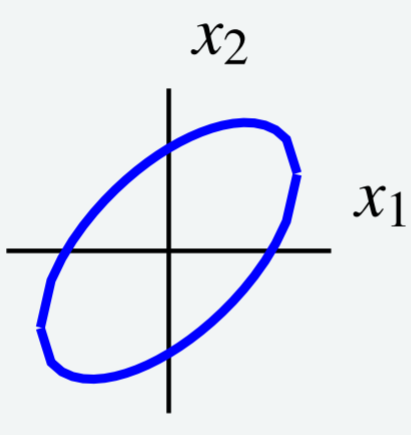
Consider the following level curve \[6x_1^2 + 4x_1x_2 + 3x_2^2 = 7\nonumber \] shown in the following graph.
Use a change of variables to choose new axes such that the ellipse is oriented parallel to the new coordinate axes. In other words, use a change of variables to rewrite \(q\) to eliminate the \(x_1x_2\) term.
Solution
Notice that the level curve is given by \(q = 7\) for \(q = 6x_1^2 + 4x_1x_2 + 3x_2^2\). This is the same quadratic form that we examined earlier in Example \(\PageIndex{13}\). Therefore we know that we can write \(q = \vec{x}^T A \vec{x}\) for the matrix \[A = \left[ \begin{array}{rr} 6 & 2 \\ 2 & 3 \end{array} \right]\nonumber \]
Now we want to orthogonally diagonalize \(A\) to write \(U^TAU=D\) for an orthogonal matrix \(U\) and diagonal matrix \(D\). The details are left to the reader, and you can verify that the resulting matrices are \[\begin{aligned} U &= \left[ \begin{array}{rr} \frac{2}{\sqrt{5}} & - \frac{1}{\sqrt{5}} \\ \frac{1}{\sqrt{5}} & \frac{2}{\sqrt{5}} \end{array} \right] \\ D &= \left[ \begin{array}{rr} 7 & 0 \\ 0 & 2 \end{array} \right]\end{aligned}\]
Next we write \(\vec{y} = \left[ \begin{array}{c} y_1 \\ y_2 \end{array} \right]\). It follows that \(\vec{x} = U \vec{y}\).
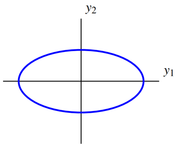
We can now express the quadratic form \(q\) in terms of \(y\), using the entries from \(D\) as coefficients as follows: \[\begin{aligned} q &= d_{11}y_1^2 + d_{22}y_2^2 \\ &= 7y_1^2 + 2y_2^2 \end{aligned}\]
Hence the level curve can be written \(7y_1^2 + 2y_2^2 =7\). The graph of this equation is given by:
The change of variables results in new axes such that with respect to the new axes, the ellipse is oriented parallel to the coordinate axes. These are called the principal axes of the quadratic form.
The following is another example of diagonalizing a quadratic form.
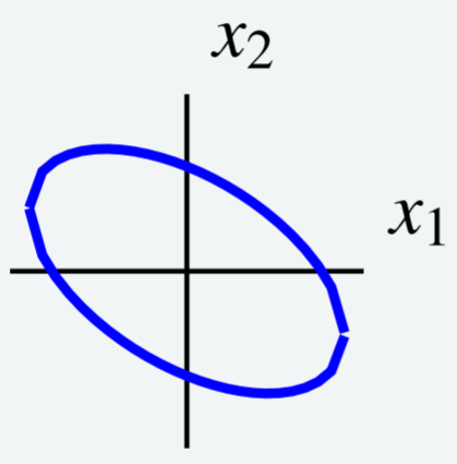
Consider the level curve \[5x_1^{2}-6x_1x_2+5x_2^{2}=8\nonumber\] shown in the following graph.
Use a change of variables to choose new axes such that the ellipse is oriented parallel to the new coordinate axes. In other words, use a change of variables to rewrite \(q\) to eliminate the \(x_1x_2\) term.
Solution
First, express the level curve as \(\vec{x}^TA\vec{x}\) where \(\vec{x} = \left[ \begin{array}{r} x_1 \\ x_2 \end{array} \right]\) and \(A\) is symmetric. Let \(A = \left[ \begin{array}{rr} a_{11} & a_{12} \\ a_{21} & a_{22} \end{array} \right]\). Then \(q = \vec{x}^T A \vec{x}\) is given by \[\begin{aligned} q &= \left[ \begin{array}{cc} x_1 & x_2 \end{array} \right] \left[ \begin{array}{rr} a_{11} & a_{12} \\ a_{21} & a_{22} \end{array} \right] \left[ \begin{array}{r} x_1 \\ x_2 \end{array} \right]\\ &= a_{11}x_1^2 + (a_{12} + a_{21})x_1x_2 + a_{22}x_2^2\end{aligned}\]
Equating this to the given description for \(q\), we have \[5x_1^2 -6x_1x_2 + 5x_2^2 = a_{11}x_1^2 + (a_{12} + a_{21})x_1x_2 + a_{22}x_2^2\nonumber \] This implies that \(a_{11} = 5, a_{22} = 5\) and in order for \(A\) to be symmetric, \(a_{12} = a_{22} = \frac{1}{2} (a_{12}+a_{21}) = -3\). The result is \(A = \left[ \begin{array}{rr} 5 & -3 \\ -3 & 5 \end{array} \right]\). We can write \(q = \vec{x}^TA\vec{x}\) as \[\left[ \begin{array}{cc} x_1 & x_2 \end{array} \right] \left[ \begin{array}{rr} 5 & -3 \\ -3 & 5 \end{array} \right] \left[ \begin{array}{c} x_1 \\ x_2 \end{array} \right] =8\nonumber \]
Next, orthogonally diagonalize the matrix \(A\) to write \(U^TAU = D\). The details are left to the reader and the necessary matrices are given by \[\begin{aligned} U &= \left[ \begin{array}{rr} \frac{1}{2}\sqrt{2} & \frac{1}{2}\sqrt{2} \\ \frac{1}{2}\sqrt{2} & - \frac{1}{2}\sqrt{2} \end{array} \right] \\ D &= \left[ \begin{array}{rr} 2 & 0 \\ 0 & 8 \end{array} \right]\end{aligned}\]
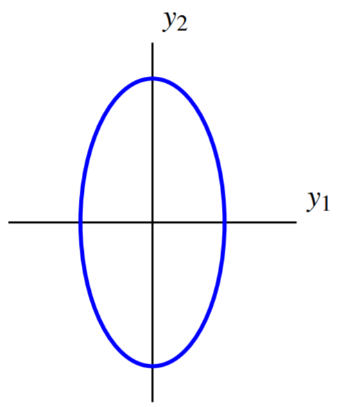
Write \(\vec{y} = \left[ \begin{array}{r} y_1 \\ y_2 \end{array} \right]\), such that \(\vec{x} = U \vec{y}\). Then it follows that \(q\) is given by \[\begin{aligned} q &= d_{11}y_1^2 + d_{22}y_2^2 \\ &= 2y_1^{2}+8y_2^{2}\end{aligned}\] Therefore the level curve can be written as \(2y_1^{2}+8y_2^{2}=8\).
This is an ellipse which is parallel to the coordinate axes. Its graph is of the form
Thus this change of variables chooses new axes such that with respect to these new axes, the ellipse is oriented parallel to the coordinate axes.