4.7: The Dot Product

Outcomes

1. Compute the dot product of vectors, and use this to compute vector projections.

The Dot Product

There are two ways of multiplying vectors which are of great importance in applications. The first of these is called the dot product. When we take the dot product of vectors, the result is a scalar. For this reason, the dot product is also called the scalar product and sometimes the inner product. The definition is as follows.

Definition \(\PageIndex{1}\): Dot Product

Let \(\vec{u},\vec{v}\) be two vectors in \(\mathbb{R}^{n}\). Then we define the dot product \(\vec{u}\bullet \vec{v}\) as \[\vec{u}\bullet \vec{v} = \sum_{k=1}^{n}u_{k}v_{k}\nonumber \]

The dot product \(\vec{u}\bullet \vec{v}\) is sometimes denoted as \((\vec{u},\vec{v})\) where a comma replaces \(\bullet\). It can also be written as \(\left\langle \vec{u},\vec{v}\right\rangle\). If we write the vectors as column or row matrices, it is equal to the matrix product \(\vec{v}\vec{w}^{T}\).

Consider the following example.

Example \(\PageIndex{1}\): Compute a Dot Product

Find \(\vec{u} \bullet \vec{v}\) for \[\vec{u} = \left[ \begin{array}{r} 1 \\ 2 \\ 0 \\ -1 \end{array} \right], \vec{v} = \left[ \begin{array}{r} 0 \\ 1 \\ 2 \\ 3 \end{array} \right]\nonumber \]

Solution

By Definition \(\PageIndex{1}\), we must compute \[\vec{u}\bullet \vec{v} = \sum_{k=1}^{4}u_{k}v_{k}\nonumber \]

This is given by \[\begin{aligned} \vec{u} \bullet \vec{v} &= (1)(0) + (2)(1) + (0)(2) + (-1)(3) \\ &= 0 + 2 + 0 + -3 \\ &= -1\end{aligned}\]

With this definition, there are several important properties satisfied by the dot product.

Proposition \(\PageIndex{1}\): Properties of the Dot Product

Let \(k\) and \(p\) denote scalars and \(\vec{u},\vec{v},\vec{w}\) denote vectors. Then the dot product \(\vec{u} \bullet \vec{v}\) satisfies the following properties.

• \(\vec{u}\bullet \vec{v}= \vec{v}\bullet \vec{u}\)
• \(\vec{u}\bullet \vec{u}\geq 0 \text{ and equals zero if and only if }\vec{u}=\vec{0}\)
• \(\left( k\vec{u}+p\vec{v}\right) \bullet \vec{w}=k\left( \vec{u}\bullet \vec{w}\right) +p\left( \vec{v}\bullet \vec{w}\right)\)
• \(\vec{u}\bullet\left( k\vec{v}+p\vec{w}\right) =k\left( \vec{u}\bullet \vec{v}\right) +p\left( \vec{u}\bullet \vec{w}\right)\)
• \(\| \vec{u}\| ^{2}=\vec{u}\bullet \vec{u}\)

Proof

The proof is left as an exercise.

This proposition tells us that we can also use the dot product to find the length of a vector.

Example \(\PageIndex{2}\): Length of a Vector

Find the length of \[\vec{u} = \left[ \begin{array}{r} 2 \\ 1 \\ 4 \\ 2 \end{array} \right]\nonumber \] That is, find \(\| \vec{u} \| .\)

Solution

By Proposition \(\PageIndex{1}\), \(\| \vec{u} \| ^{2} = \vec{u} \bullet \vec{u}\). Therefore, \(\| \vec{u} \| = \sqrt {\vec{u} \bullet \vec{u}}\). First, compute \(\vec{u} \bullet \vec{u}\).

This is given by \[\begin{aligned} \vec{u} \bullet \vec{u} &= (2)(2) + (1)(1) + (4)(4) + (2)(2) \\ &= 4 + 1 + 16 + 4 \\ &= 25\end{aligned}\]

Then, \[\begin{aligned} \| \vec{u} \| &= \sqrt {\vec{u} \bullet \vec{u}} \\ &= \sqrt{25} \\ &= 5\end{aligned}\]

You may wish to compare this to our previous definition of length, given in Definition 4.4.2.

The Cauchy Schwarz inequality is a fundamental inequality satisfied by the dot product. It is given in the following theorem.

Theorem \(\PageIndex{1}\): Cauchy Schwarz Inequality

The dot product satisfies the inequality \[\left\vert \vec{u}\bullet \vec{v}\right\vert \leq \| \vec{u}\| \| \vec{v}\| \label{cauchy}\] Furthermore equality is obtained if and only if one of \(\vec{u}\) or \(\vec{v}\) is a scalar multiple of the other.

Proof

First note that if \(\vec{v}=\vec{0}\) both sides of \(\eqref{cauchy}\) equal zero and so the inequality holds in this case. Therefore, it will be assumed in what follows that \(\vec{v}\neq \vec{0}\).

Define a function of \(t\in \mathbb{R}\) by \[f\left( t\right) =\left( \vec{u}+t\vec{v}\right) \bullet \left( \vec{u}+ t\vec{v}\right)\nonumber \] Then by Proposition \(\PageIndex{1}\), \(f\left( t\right) \geq 0\) for all \(t\in \mathbb{R}\). Also from Proposition \(\PageIndex{1}\) \[\begin{aligned} f\left( t\right) &=\vec{u}\bullet \left( \vec{u}+t\vec{v}\right) + t\vec{v}\bullet \left( \vec{u}+t\vec{v}\right) \\ &=\vec{u}\bullet \vec{u}+t\left( \vec{u}\bullet \vec{v}\right) + t \vec{v}\bullet \vec{u}+ t^{2}\vec{v}\bullet \vec{v} \\ &=\| \vec{u}\| ^{2}+2t\left( \vec{u}\bullet \vec{v}\right) +\| \vec{v}\| ^{2}t^{2}\end{aligned}\]

Now this means the graph of \(y=f\left( t\right)\) is a parabola which opens up and either its vertex touches the \(t\) axis or else the entire graph is above the \(t\) axis. In the first case, there exists some \(t\) where \(f\left( t\right) =0\) and this requires \(\vec{u}+t\vec{v}=\vec{0}\) so one vector is a multiple of the other. Then clearly equality holds in \(\eqref{cauchy}\). In the case where \(\vec{v}\) is not a multiple of \(\vec{u}\), it follows \(f\left( t\right) >0\) for all \(t\) which says \(f\left( t\right)\) has no real zeros and so from the quadratic formula, \[\left( 2\left( \vec{u}\bullet \vec{v}\right) \right) ^{2}-4\| \vec{u} \| ^{2}\| \vec{v}\| ^{2}<0\nonumber \] which is equivalent to \(\left\vert \vec{u}\bullet \vec{v} \right\vert <\| \vec{u}\| \| \vec{v}\|\).

Notice that this proof was based only on the properties of the dot product listed in Proposition \(\PageIndex{1}\). This means that whenever an operation satisfies these properties, the Cauchy Schwarz inequality holds. There are many other instances of these properties besides vectors in \(\mathbb{R}^{n}\).

The Cauchy Schwarz inequality provides another proof of the triangle inequality for distances in \(\mathbb{R}^{n}\).

Theorem \(\PageIndex{2}\): Triangle Inequality

For \(\vec{u},\vec{v}\in \mathbb{R}^{n}\) \[\| \vec{u}+\vec{v}\| \leq \| \vec{u}\| +\| \vec{v} \| \label{triangleineq1}\] and equality holds if and only if one of the vectors is a non-negative scalar multiple of the other.

Also \[\| \| \vec{u}\| -\| \vec{v}\| \| \leq \| \vec{u}-\vec{v}\| \label{triangleineq2}\]

Proof

By properties of the dot product and the Cauchy Schwarz inequality, \[\begin{aligned} \| \vec{u}+\vec{v}\| ^{2} &= \left( \vec{u}+\vec{v}\right) \bullet \left( \vec{u}+\vec{v}\right) \\ & =\left( \vec{u}\bullet \vec{u}\right) +\left( \vec{u}\bullet \vec{v}\right) +\left(\vec{v}\bullet \vec{u}\right) +\left( \vec{v}\bullet \vec{v}\right) \\ &=\| \vec{u}\| ^{2}+2\left( \vec{u}\bullet \vec{v}\right)+\| \vec{v}\| ^{2} \\ &\leq \| \vec{u}\| ^{2}+2\left\vert \vec{u}\bullet \vec{v}\right\vert +\| \vec{v}\| ^{2} \\ &\leq \| \vec{u}\| ^{2}+2\| \vec{u}\| \| \vec{v}\| +\| \vec{v}\| ^{2} =\left( \| \vec{u}\| +\| \vec{v}\|\right) ^{2}\end{aligned}\] Hence, \[\| \vec{u}+\vec{v}\| ^{2} \leq \left( \| \vec{u}\| +\| \vec{v}\| \right) ^{2}\nonumber \] Taking square roots of both sides you obtain \(\eqref{triangleineq1}\).

It remains to consider when equality occurs. Suppose \(\vec{u} = \vec{0}\). Then, \(\vec{u} = 0 \vec{v}\) and the claim about when equality occurs is verified. The same argument holds if \(\vec{v} = \vec{0}\). Therefore, it can be assumed both vectors are nonzero. To get equality in \(\eqref{triangleineq1}\) above, Theorem \(\PageIndex{1}\) implies one of the vectors must be a multiple of the other. Say \(\vec{v}= k \vec{u}\). If \(k <0\) then equality cannot occur in \(\eqref{triangleineq1}\) because in this case \[\vec{u}\bullet \vec{v} =k \| \vec{u}\| ^{2}<0<\left| k \right| \| \vec{u}\| ^{2}=\left| \vec{u}\bullet \vec{v}\right|\nonumber \] Therefore, \(k \geq 0.\)

To get the other form of the triangle inequality write \[\vec{u}=\vec{u}-\vec{v}+\vec{v}\nonumber \] so \[\begin{aligned} \| \vec{u}\| & =\| \vec{u}-\vec{v}+\vec{v}\| \\ & \leq \| \vec{u}-\vec{v}\| +\| \vec{v}\| \end{aligned}\] Therefore, \[\| \vec{u}\| -\| \vec{v}\| \leq \| \vec{u}-\vec{v} \| \label{triangleineq3}\] Similarly, \[\| \vec{v}\| -\| \vec{u}\| \leq \| \vec{v}-\vec{u} \| =\| \vec{u}-\vec{v}\| \label{triangleineq4}\] It follows from \(\eqref{triangleineq3}\) and \(\eqref{triangleineq4}\) that \(\eqref{triangleineq2}\) holds. This is because \(\left| \| \vec{u}\| -\| \vec{v}\| \right|\) equals the left side of either \(\eqref{triangleineq3}\) or \(\eqref{triangleineq4}\) and either way, \(\left| \| \vec{u}\| -\| \vec{v}\| \right| \leq \| \vec{u}-\vec{v}\|\).

The Geometric Significance of the Dot Product

Given two vectors, \(\vec{u}\) and \(\vec{v}\), the included angle is the angle between these two vectors which is given by \(\theta\) such that \(0 \leq \theta \leq \pi\). The dot product can be used to determine the included angle between two vectors. Consider the following picture where \(\theta\) gives the included angle.

Figure \(\PageIndex{1}\)

Proposition \(\PageIndex{2}\): The Dot Product and the Included Angle

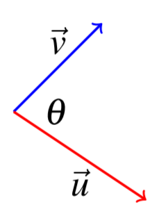
Let \(\vec{u}\) and \(\vec{v}\) be two vectors in \(\mathbb{R}^n\), and let \(\theta\) be the included angle. Then the following equation holds. \[\vec{u}\bullet \vec{v}=\| \vec{u}\| \| \vec{v} \| \cos \theta\nonumber \]

In words, the dot product of two vectors equals the product of the magnitude (or length) of the two vectors multiplied by the cosine of the included angle. Note this gives a geometric description of the dot product which does not depend explicitly on the coordinates of the vectors.

Consider the following example.

Example \(\PageIndex{3}\): Find the Angle Between Two Vectors

Find the angle between the vectors given by \[\vec{u} = \left[ \begin{array}{r} 2 \\ 1 \\ -1 \end{array} \right], \vec{v} = \left[ \begin{array}{r} 3 \\ 4 \\ 1 \end{array} \right]\nonumber \]

Solution

By Proposition \(\PageIndex{2}\), \[\vec{u}\bullet \vec{v}=\| \vec{u}\| \| \vec{v} \| \cos \theta\nonumber \] Hence, \[\cos \theta =\frac{\vec{u}\bullet \vec{v}}{\| \vec{u}\| \| \vec{v} \|}\nonumber \]

First, we can compute \(\vec{u}\bullet \vec{v}\). By Definition \(\PageIndex{1}\), this equals \[\vec{u}\bullet \vec{v} = (2)(3) + (1)(4)+(-1)(1) = 9\nonumber \]

Then, \[\begin{array}{c} \| \vec{u} \| = \sqrt{(2)(2)+(1)(1)+(1)(1)}=\sqrt{6}\\ \| \vec{v} \| = \sqrt{(3)(3)+(4)(4)+(1)(1)}=\sqrt{26} \end{array}\nonumber \] Therefore, the cosine of the included angle equals \[\cos \theta =\frac{9}{\sqrt{26}\sqrt{6}}=0.7205766...\nonumber \]

With the cosine known, the angle can be determined by computing the inverse cosine of that angle, giving approximately \(\theta =0.76616\) radians.

Another application of the geometric description of the dot product is in finding the angle between two lines. Typically one would assume that the lines intersect. In some situations, however, it may make sense to ask this question when the lines do not intersect, such as the angle between two object trajectories. In any case we understand it to mean the smallest angle between (any of) their direction vectors. The only subtlety here is that if \(\vec{u}\) is a direction vector for a line, then so is any multiple \(k\vec{u}\), and thus we will find complementary angles among all angles between direction vectors for two lines, and we simply take the smaller of the two.

Example \(\PageIndex{4}\): Find the Angle Between Two Lines

Find the angle between the two lines \[L_1: \; \left[ \begin{array}{r} x \\ y \\ z \end{array} \right] = \left[ \begin{array}{r} 1 \\ 2 \\ 0 \end{array} \right] +t\left[ \begin{array}{r} -1 \\ 1 \\ 2 \end{array} \right]\nonumber \] and \[L_2: \; \left[ \begin{array}{r} x \\ y \\ z \end{array} \right] = \left[ \begin{array}{r} 0 \\ 4 \\ -3 \end{array} \right] +s\left[ \begin{array}{r} 2 \\ 1 \\ -1 \end{array} \right]\nonumber \]

Solution

You can verify that these lines do not intersect, but as discussed above this does not matter and we simply find the smallest angle between any directions vectors for these lines.

To do so we first find the angle between the direction vectors given above: \[\vec{u}=\left[ \begin{array}{r} -1 \\ 1 \\ 2 \end{array} \right],\; \vec{v}=\left[ \begin{array}{r} 2 \\ 1 \\ -1 \end{array} \right]\nonumber \]

In order to find the angle, we solve the following equation for \(\theta\) \[\vec{u}\bullet \vec{v}=\| \vec{u}\| \| \vec{v} \| \cos \theta\nonumber \] to obtain \(\cos \theta = -\frac{1}{2}\) and since we choose included angles between \(0\) and \(\pi\) we obtain \(\theta = \frac{2 \pi}{3}\).

Now the angles between any two direction vectors for these lines will either be \(\frac{2 \pi}{3}\) or its complement \(\phi = \pi - \frac{2 \pi}{3} = \frac{\pi}{3}\). We choose the smaller angle, and therefore conclude that the angle between the two lines is \(\frac{\pi}{3}\).

We can also use Proposition \(\PageIndex{2}\) to compute the dot product of two vectors.

Example \(\PageIndex{5}\): Using Geometric Description to Find a Dot Product

Let \(\vec{u},\vec{v}\) be vectors with \(\| \vec{u} \| = 3\) and \(\| \vec{v} \| = 4\). Suppose the angle between \(\vec{u}\) and \(\vec{v}\) is \(\pi / 3\). Find \(\vec{u}\bullet \vec{v}\).

Solution

From the geometric description of the dot product in Proposition \(\PageIndex{2}\) \[\vec{u}\bullet \vec{v}=(3)(4) \cos \left( \pi / 3\right) =3\times 4\times 1/2=6\nonumber \]

Two nonzero vectors are said to be perpendicular, sometimes also called orthogonal, if the included angle is \(\pi /2\) radians (\(90^{\circ }).\)

Consider the following proposition.

Proposition \(\PageIndex{3}\): Perpendicular Vectors

Let \(\vec{u}\) and \(\vec{v}\) be nonzero vectors in \(\mathbb{R}^n\). Then, \(\vec{u}\) and \(\vec{v}\) are said to be perpendicular exactly when \[\vec{u} \bullet \vec{v} = 0\nonumber \]

Proof

This follows directly from Proposition \(\PageIndex{2}\). First if the dot product of two nonzero vectors is equal to \(0\), this tells us that \(\cos \theta =0\) (this is where we need nonzero vectors). Thus \(\theta = \pi /2\) and the vectors are perpendicular.

If on the other hand \(\vec{v}\) is perpendicular to \(\vec{u}\), then the included angle is \(\pi /2\) radians. Hence \(\cos \theta =0\) and \(\vec{u} \bullet \vec{v} = 0\).

Consider the following example.

Example \(\PageIndex{6}\): Determine if Two Vectors are Perpendicular

Determine whether the two vectors, \[\vec{u}= \left[ \begin{array}{r} 2 \\ 1 \\ -1 \end{array} \right], \vec{v} = \left[ \begin{array}{r} 1 \\ 3 \\ 5 \end{array} \right]\nonumber \] are perpendicular.

Solution

In order to determine if these two vectors are perpendicular, we compute the dot product. This is given by \[\vec{u} \bullet \vec{v} = (2)(1) + (1)(3) + (-1)(5) = 0\nonumber \] Therefore, by Proposition \(\PageIndex{3}\) these two vectors are perpendicular.

Projections

In some applications, we wish to write a vector as a sum of two related vectors. Through the concept of projections, we can find these two vectors. First, we explore an important theorem. The result of this theorem will provide our definition of a vector projection.

Theorem \(\PageIndex{3}\): Vector Projections

Let \(\vec{v}\) and \(\vec{u}\) be nonzero vectors. Then there exist unique vectors \(\vec{v}_{||}\) and \(\vec{v}_{\bot }\) such that \[\vec{v}=\vec{v}_{||}+\vec{v}_{\bot } \label{projection}\] where \(\vec{v}_{||}\) is a scalar multiple of \(\vec{u}\), and \(\vec{v}_{\bot}\) is perpendicular to \(\vec{u}\).

Proof

Suppose \(\eqref{projection}\) holds and \(\vec{v}_{||}= k \vec{u}\). Taking the dot product of both sides of \(\eqref{projection}\) with \(\vec{u}\) and using \(\vec{v}_{\bot }\bullet \vec{u}=0,\) this yields \[\begin{array}{ll} \vec{v}\bullet \vec{u} & = ( \vec{v}_{||}+\vec{v}_{\bot }) \bullet \vec{u} \\ & = k\vec{u} \bullet \vec{u} + \vec{v}_{\bot} \bullet \vec{u} \\ & = k \| \vec{u}\| ^{2} \end{array}\nonumber \] which requires \(k =\vec{v}\bullet \vec{u} / \| \vec{u}\| ^{2}.\) Thus there can be no more than one vector \(\vec{v}_{||}\). It follows \(\vec{v}_{\bot }\) must equal \(\vec{v}-\vec{v}_{||}.\) This verifies there can be no more than one choice for both \(\vec{v}_{||}\) and \(\vec{v}_{\bot }\) and proves their uniqueness.

Now let \[\vec{v}_{||} = \frac{\vec{v}\bullet \vec{u}}{\| \vec{u}\| ^{2}}\vec{u}\nonumber \] and let \[\vec{v}_{\bot }=\vec{v}-\vec{v}_{||}=\vec{v}-\frac{\vec{v}\bullet \vec{u}} {\| \vec{u}\| ^{2}}\vec{u}\nonumber \] Then \(\vec{v}_{||}= k\vec{u}\) where \(k =\frac{\vec{v}\bullet \vec{u}}{\| \vec{u}\| ^{2}}\). It only remains to verify \(\vec{v}_{\bot }\bullet \vec{u}=0.\) But \[\begin{aligned} \vec{v}_{\bot }\bullet \vec{u} &= \vec{v}\bullet \vec{u}-\frac{\vec{v}\bullet \vec{u}}{\| \vec{u}\| ^{2}}\vec{u}\bullet \vec{u} \\ &= \vec{v}\bullet\vec{u}-\vec{v}\bullet \vec{u}\\ &= 0 \end{aligned}\]

The vector \(\vec{v}_{||}\) in Theorem \(\PageIndex{3}\) is called the projection of \(\vec{v}\) onto \(\vec{u}\) and is denoted by \[\vec{v}_{||} = \mathrm{proj}_{\vec{u}}\left( \vec{v}\right)\nonumber \]

We now make a formal definition of the vector projection.

Definition \(\PageIndex{2}\): Vector Projection

Let \(\vec{u}\) and \(\vec{v}\) be vectors. Then, the projection of \(\vec{v}\) onto \(\vec{u}\) is given by \[\mathrm{proj}_{\vec{u}}\left( \vec{v}\right) =\left( \frac{\vec{v}\bullet \vec{u}}{\vec{u}\bullet \vec{u}}\right) \vec{u} = \frac{\vec{v}\bullet \vec{u}}{\| \vec{u}\| ^{2}}\vec{u}\nonumber \]

Consider the following example of a projection.

Example \(\PageIndex{7}\): Find the Projection of One Vector Onto Another

Find \(\mathrm{proj}_{\vec{u}}\left( \vec{v}\right)\) if \[\vec{u}= \left[ \begin{array}{r} 2 \\ 3 \\ -4 \end{array} \right], \vec{v}= \left[ \begin{array}{r} 1 \\ -2 \\ 1 \end{array} \right]\nonumber \]

Solution

We can use the formula provided in Definition \(\PageIndex{2}\) to find \(\mathrm{proj}_{\vec{u}}\left( \vec{v}\right)\). First, compute \(\vec{v} \bullet \vec{u}\). This is given by \[\begin{aligned} \left[ \begin{array}{r} 1 \\ -2 \\ 1 \end{array} \right] \bullet \left[ \begin{array}{r} 2 \\ 3 \\ -4 \end{array} \right] &= (2)(1) + (3)(-2) + (-4)(1) \\ &= 2 - 6 - 4 \\ &= -8\end{aligned}\] Similarly, \(\vec{u} \bullet \vec{u}\) is given by \[\begin{aligned} \left[ \begin{array}{r} 2 \\ 3 \\ -4 \end{array} \right] \bullet \left[ \begin{array}{r} 2 \\ 3 \\ -4 \end{array} \right] &= (2)(2) + (3)(3) + (-4)(-4) \\ &= 4 + 9 + 16 \\ &= 29\end{aligned}\]

Therefore, the projection is equal to \[\begin{aligned} \mathrm{proj}_{\vec{u}}\left( \vec{v}\right) &=-\frac{8}{29} \left[ \begin{array}{r} 2 \\ 3 \\ -4 \end{array} \right] \\ &= \left[ \begin{array}{r} - \frac{16}{29} \\ - \frac{24}{29} \\ \frac{32}{29} \end{array} \right]\end{aligned}\]

We will conclude this section with an important application of projections. Suppose a line \(L\) and a point \(P\) are given such that \(P\) is not contained in \(L\). Through the use of projections, we can determine the shortest distance from \(P\) to \(L\).

Example \(\PageIndex{8}\): Shortest Distance from a Point to a Line

Let \(P = (1,3,5)\) be a point in \(\mathbb{R}^3\), and let \(L\) be the line which goes through point \(P_0 = (0,4,-2)\) with direction vector \(\vec{d} = \left[ \begin{array}{r} 2 \\ 1 \\ 2 \end{array} \right]\). Find the shortest distance from \(P\) to the line \(L\), and find the point \(Q\) on \(L\) that is closest to \(P\).

Solution

In order to determine the shortest distance from \(P\) to \(L\), we will first find the vector \(\overrightarrow{P_0P}\) and then find the projection of this vector onto \(L\). The vector \(\overrightarrow{P_0P}\) is given by \[\left[ \begin{array}{r} 1 \\ 3 \\ 5 \end{array} \right] - \left[ \begin{array}{r} 0 \\ 4 \\ -2 \end{array} \right] = \left[ \begin{array}{r} 1 \\ -1 \\ 7 \end{array} \right]\nonumber \]

Then, if \(Q\) is the point on \(L\) closest to \(P\), it follows that \[\begin{aligned} \overrightarrow{P_0Q} &= \mathrm{proj}_{\vec{d}}\overrightarrow{P_0P} \\ &= \left( \frac{ \overrightarrow{P_0P}\bullet \vec{d}}{\|\vec{d}\|^2}\right) \vec{d} \\ &= \frac{15}{9} \left[ \begin{array}{r} 2 \\ 1 \\ 2 \end{array} \right] \\ &= \frac{5}{3} \left[ \begin{array}{r} 2 \\ 1 \\ 2 \end{array} \right]\end{aligned}\]

Now, the distance from \(P\) to \(L\) is given by \[\| \overrightarrow{QP} \| = \| \overrightarrow{P_0P} - \overrightarrow{P_0Q}\| = \sqrt{26}\nonumber \]

The point \(Q\) is found by adding the vector \(\overrightarrow{P_0Q}\) to the position vector \(\overrightarrow{0P_0}\) for \(P_0\) as follows \[\begin{aligned} \left[ \begin{array}{r} 0 \\ 4 \\ -2 \end{array} \right] + \frac{5}{3} \left[ \begin{array}{r} 2 \\ 1 \\ 2 \end{array} \right] &= \left[ \begin{array}{r} \frac{10}{3} \\ \frac{17}{3} \\ \frac{4}{3} \end{array} \right]\end{aligned}\]

Therefore, \(Q = (\frac{10}{3}, \frac{17}{3}, \frac{4}{3})\).