1.1: Nerve Fibers and the Strang Quartet
- Page ID
- 21798

We wish to confirm, by example, the prefatory claim that matrix algebra is a useful means of organizing (stating and solving) multivariable problems. In our first such example we investigate the response of a nerve fiber to a constant current stimulus. Ideally, a nerve fiber is simply a cylinder of radius aa and length \(l\) that conducts electricity both along its length and across its lateral membrane. Though we shall, in subsequent chapters, delve more deeply into the biophysics, here, in our first outing, we shall stick to its purely resistive properties. The latter are expressed via two quantities:
- \(\rho_{i}\) the resistivity in \(\Omega cm\) of the cytoplasm that fills the cell, and
- \(\rho_{m}\) the resistivity in \(\Omega cm^{2}\) of the cell's lateral membrane.
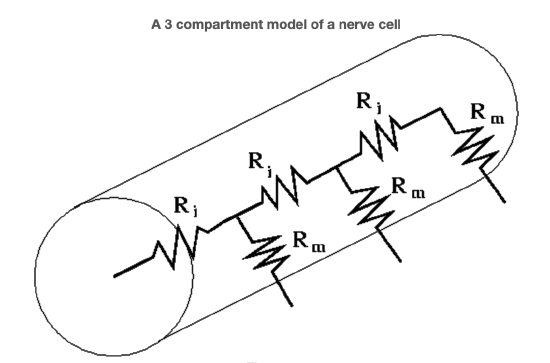
Although current surely varies from point to point along the fiber it is hoped that these variations are regular enough to be captured by a multicompartment model. By that we mean that we choose a number \(N\) and divide the fiber into \(N\) segments each of length \(\frac{l}{N}\) Denoting a segment's axial resistance
\[R_{i} = \frac{\rho_{i} \frac{l}{N}}{\pi a^2} \nonumber\]
and membrane resistance
\[R_{m} = \frac{\rho_{m}}{2\pi a \frac{l}{N}} \nonumber\]
we arrive at the lumped circuit model of Figure 1. For a fiber in culture we may assume a constant extracellular potential, e.g., zero. We accomplish this by connecting and grounding the extracellular nodes, see Figure 2.
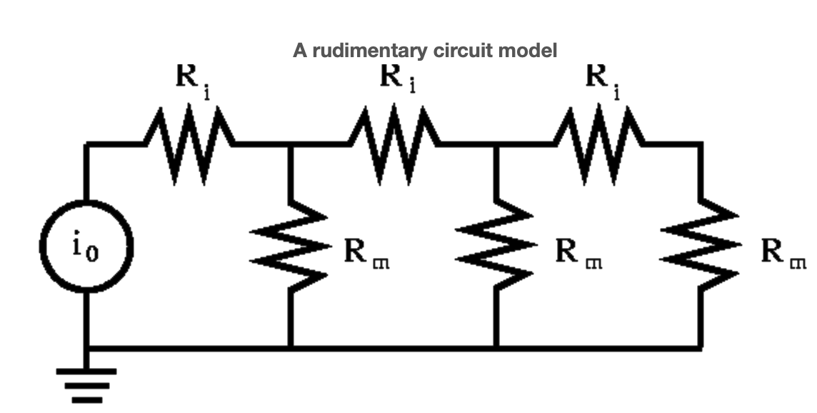
Figure 2 also incorporates the exogenous disturbance, a current stimulus between ground and the left end of the fiber. Our immediate goal is to compute the resulting currents through each resistor and the potential at each of the nodes. Our long--range goal is to provide a modeling methodology that can be used across the engineering and science disciplines. As an aid to computing the desired quantities we give them names. With respect to figure 3, we label the vector of potentials
\[x = \begin{pmatrix} {x_{1}}&{x_{2}}&{x_{3}}&{x_{4}} \end{pmatrix} \nonumber\]
\[y = \begin{pmatrix} {y_{1}}&{y_{2}}&{y_{3}}&{y_{4}}&{y_{5}}&{y_{6}} \end{pmatrix} \nonumber\]
We have also (arbitrarily) assigned directions to the currents as a graphical aid in the consistent application of the basic circuit laws.
We incorporate the circuit laws in a modeling methodology that takes the form of a Strang Quartet:
- (S1) Express the voltage drops via \(\textbf{e} = -(A \textbf{x})\)
- (S2) Express Ohm's Law via \(\textbf{y} = G \textbf{e}\)
- (S3) Express Kirchhoff's Current Law via \(A^{T} \textbf{y} = -\textbf{f}\)
- (S4) Combine the above into \(A^{T}GA \textbf{x} = \textbf{f}\)
The \(A\) in (S1) is the node-edge adjacency matrix -- it encodes the network's connectivity. The \(G\) in (S2) is the diagonal matrix of edge conductances -- it encodes the physics of the network. The \(\textbf{f}\) in (S3) is the vector of current sources -- it encodes the network's stimuli. The culminating \(A^{T}GA\) in (S4) is the symmetric matrix whose inverse, when applied to \(\textbf{f}\), reveals the vector of potentials, \(\textbf{x}\). In order to make these ideas our own we must work many, many examples.
Strang Quartet, Step 1
With respect to the circuit of Figure 3, in accordance with step 1, we express the six potential differences (always tail minus head)
\[e_{1} = x_{1}-x_{2} \nonumber\]
\[e_{2} = x_{2} \nonumber\]
\[e_{3} = x_{2}-x_{3} \nonumber\]
\[e_{4} = x_{3} \nonumber\]
\[e_{5} = x_{3}-x_{4} \nonumber\]
\[e_{6} = x_{4} \nonumber\]
Such long, tedious lists cry out for matrix representation, to wit \( \textbf{e} = -(A \textbf{x})\) where
\[A = \begin{pmatrix} {-1}&{1}&{0}&{0}\\ {0}&{-1}&{0}&{0}\\ {0}&{-1}&{1}&{0}\\ {0}&{0}&{-1}&{0}\\ {0}&{0}&{-1}&{1}\\ {0}&{0}&{0}&{-1}\\ \end{pmatrix} \nonumber\]
Strang Quartet, Step 2
Step 2, Ohm's Law, states:
The current along an edge is equal to the potential drop across the edge divided by the resistance of the edge.
In our case,
\[\begin{array}{ccccc} {y_{j} = \frac{e_{j}}{R_{i}},}&{j = 1, 3, 5}&{and}&{y_{j} = \frac{e_{j}}{R_{m}},}&{j = 2, 4, 6} \nonumber \end{array}\]
or, in matrix notation, \(\textbf{y} = G \textbf{e}\) where
\[A = \begin{pmatrix} {\frac{1}{R_{i}}}&{0}&{0}&{0}&{0}&{0}\\ {0}&{\frac{1}{R_{m}}}&{0}&{0}&{0}&{0}\\ {0}&{0}&{\frac{1}{R_{i}}}&{0}&{0}&{0}\\ {0}&{0}&{0}&{\frac{1}{R_{m}}}&{0}&{0}\\ {0}&{0}&{0}&{0}&{\frac{1}{R_{i}}}&{0}\\ {0}&{0}&{0}&{0}&{0}&{\frac{1}{R_{m}}}\\ \end{pmatrix} \nonumber\]
Strang Quartet, Step 3
Step 3, Kirchhoff's Current Law, states:
The sum of the currents into each node must be zero.
In our case
\[i_{0}-y_{1}=0 \nonumber\]
\[y_{1}-y_{2}-y_{3} = 0 \nonumber\]
\[y_{3}-y_{4}-y_{5} = 0 \nonumber\]
\[y_{5}-y_{6} = 0 \nonumber\]
or, in matrix terms
\[B \textbf{y} = -\textbf{f} \nonumber\]
where
\[\begin{array}{ccc} {B = \begin{pmatrix} {-1}&{0}&{0}&{0}&{0}&{0}\\ {1}&{-1}&{-1}&{0}&{0}&{0}\\ {0}&{0}&{1}&{-1}&{-1}&{0}\\ {0}&{0}&{0}&{0}&{1}&{-1}\\ \end{pmatrix}}&{and}&{f = \begin{pmatrix} {i_{0}}\\ {0}\\ {0}\\ {0} \end{pmatrix}} \nonumber \end{array}\]
Strang Quartet, Step 4
Looking back at A
\[A = \begin{pmatrix} {-1}&{1}&{0}&{0}\\ {0}&{-1}&{0}&{0}\\ {0}&{-1}&{1}&{0}\\ {0}&{0}&{-1}&{0}\\ {0}&{0}&{-1}&{1}\\ {0}&{0}&{0}&{-1}\\ \end{pmatrix} \nonumber\]
we recognize in B the transpose of A
- (S1) \(\textbf{e} = -(A \textbf{x})\)
- (S2) \(\textbf{y} = G \textbf{e}\)
- (S3) \(A^{T} \textbf{y} = -\textbf{f}\)
On substitution of the first two into the third we arrive, in accordance with (S4), at
\(A^{T}GA \textbf{x} = \textbf{f}\)
This is a system of four equations for the 4 unknown potentials, \(x_{1}\) through \(x_{4}\) As you know, the system Equation may have either 1, 0, or infinitely many solutions, depending on \(\textbf{f}\) and \(A^{T}GA\) We shall devote (FIX ME CNXN TO CHAPTER 3 AND 4) to an unraveling of the previous sentence. For now, we cross our fingers and 'solve' by invoking the Matlab program
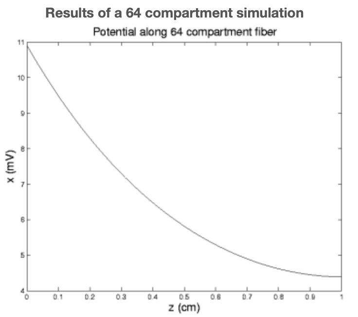
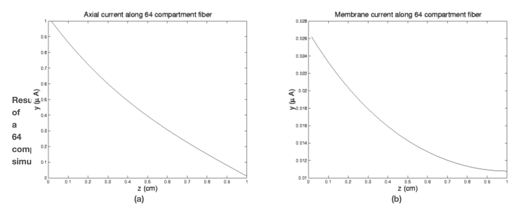
Figure 5.
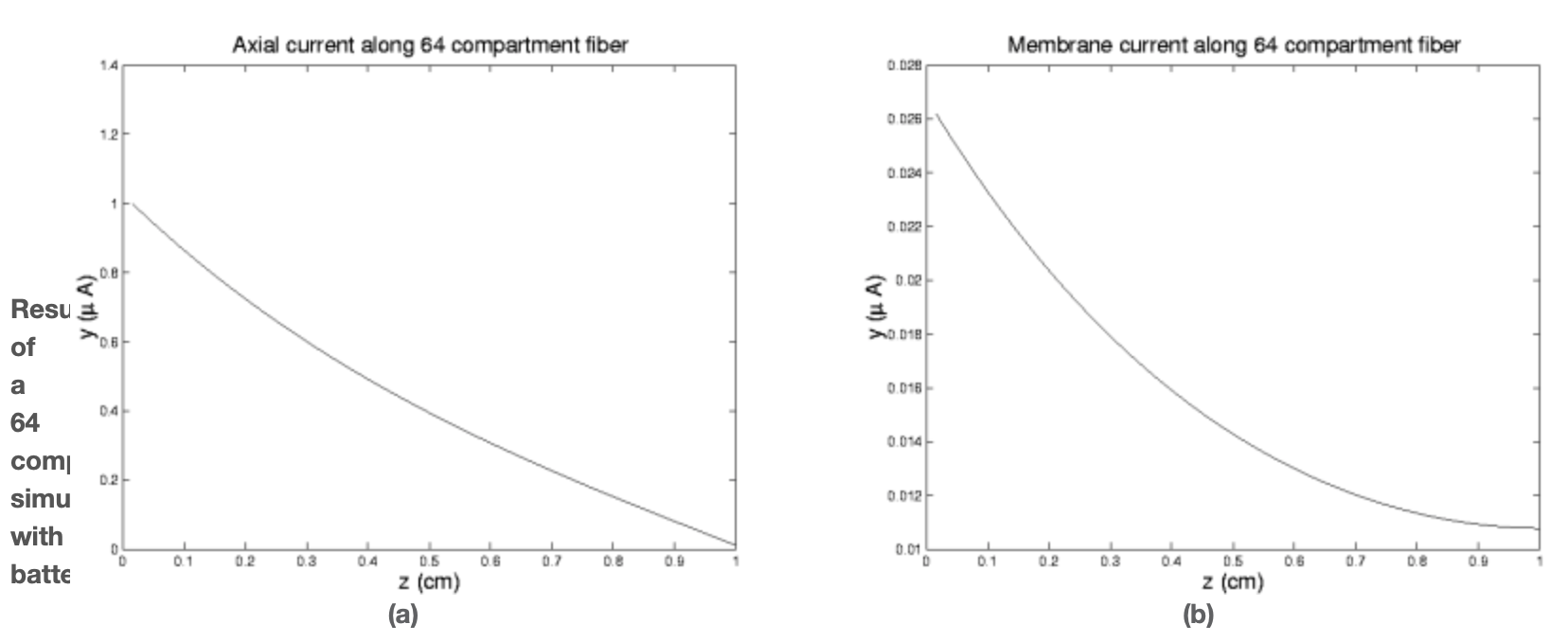
This program is a bit more ambitious than the above in that it allows us to specify the number of compartments and that rather than just spewing the x and y values it plots them as a function of distance along the fiber. We note that, as expected, everything tapers off with distance from the source and that the axial current is significantly greater than the membrane, or leakage, current.
We have seen in the previous example how a current source may produce a potential difference across a cell's membrane. We note that, even in the absence of electrical stimuli, there is always a difference in potential between the inside and outside of a living cell. In fact, this difference is the biologist's definition of 'living.' Life is maintained by the fact that the cell's interior is rich in potassium ions, \(K^{+}\) and poor in sodium ions, \(Na^{+}\) while in the exterior medium it is just the opposite. These concentration differences beget potential differences under the guise of the Nernst potentials:
- Nernst potentials
\[\begin{array}{ccc} {E_{Na} = \frac{RT}{F} \log \frac{[Na]_{o}}{[Na]_{i}}}&{and}&{E_{K} = \frac{RT}{F} \log \frac{[K]_{o}}{[K]_{i}}} \nonumber \end{array}\]
where R is the gas constant, T is temperature, and F is the Faraday constant.Associated with these potentials are membrane resistances
\[\begin{array}{ccc} {\rho_{m, Na}}&{and}&{\rho_{m,K}} \nonumber \end{array}\]
that together produce the \(\rho_{m}\) above via
\[\frac{1}{\rho_{m}} = \frac{1}{\rho_{m, Na}}+\frac{1}{\rho_{m,K}} \nonumber\]
and produce the aforementioned rest potential
\[E_{m} = \rho_{m}(\frac{E_{Na}}{\rho_{m, Na}}+\frac{E_{K}}{\rho_{m,K}} \nonumber\]
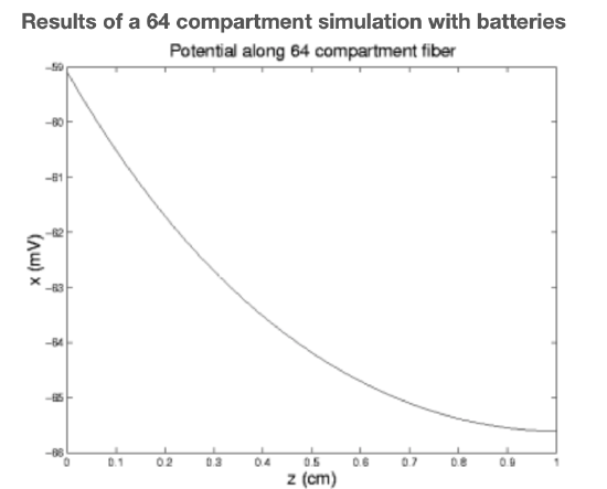
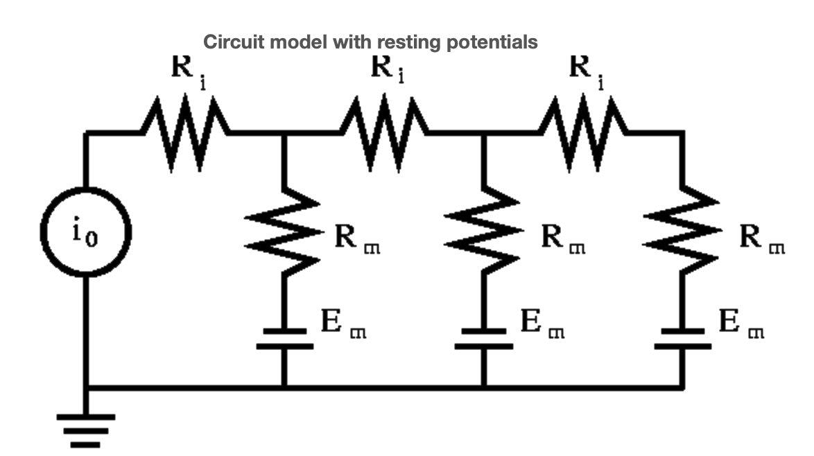
With respect to our old circuit model, each compartment now sports a battery in series with its membrane resistance, as shown in Figure 6.
Revisiting step (S1-4) we note that in (S1) the even numbered voltage drops are now
\[e_{2} = x_{2}-E_{m} \nonumber\]
\[e_{4} = x_{3}-E_{m} \nonumber\]
\[e_{6} = x_{4}-E_{m} \nonumber\]
We accommodate such things by generalizing (S1) to:
- (S1') Express the voltage drops as \(e = \textbf{b}-A \textbf{x}\) where \(\textbf{b}\) is the vector of batteries.
No changes are necessary for (S2) and (S3). The final step now reads,
- (S4') Combine (S1'), (S2), and (S3) to produce \(A^{T}GA \textbf{x} = A^{T}G \textbf{b} \textbf{f}\)
Returning to Figure 6, we note that
\[\begin{array}{ccc} {\textbf{b} = -\begin{pmatrix} E_{m} \begin{pmatrix} {0}\\ {1}\\ {0}\\ {1}\\ {0}\\ {1} \end{pmatrix} \end{pmatrix}}&{and}&{A^{T}G \textbf{b} = \frac{E_{m}}{R_{m}} \begin{pmatrix} {0}\\ {1}\\ {1}\\ {1} \end{pmatrix}} \nonumber \end{array}\]
This requires only minor changes to our old code. The results of its use are indicated in the next two figures.