
2.1: A Uniaxial Truss
- Page ID
- 21805

Introduction
We now investigate the mechanical prospection of tissue, an application extending techniques developed in the electrical analysis of a nerve cell. In this application, one applies traction to the edges of a square sample of planar tissue and seeks to identify, from measurement of the resulting deformation, regions of increased 'hardness' or 'stiffness.'
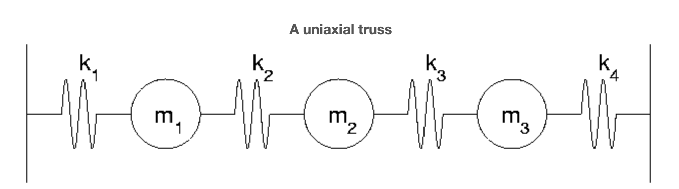
As a precursor to the biaxial problem let us first consider the uniaxial case. We connect 3 masses with four springs between two immobile walls, apply forces at the masses, and measure the associated displacement. More precisely, we suppose that a horizontal force, \(f_{j}\) is applied to each \(m_{j}\) and produces a displacement \(x_{j}\) with the sign convention that rightward means positive. The bars at the ends of the figure indicate rigid supports incapable of movement. The \(k_{j}\) denote the respective spring stiffnesses. The analog of potential difference (see the electrical model) is here elongation. If \(e_{j}\) denotes the elongation of the jth spring then naturally,
\[e_{1} = x_{1} \nonumber\]
\[e_{2} = x_{2}-x_{1} \nonumber\]
\[e_{3} = x_{3}-x_{2} \nonumber\]
\[e_{4} = -x_{3} \nonumber\]
or, in matrix terms, \(\textbf{e} = A \textbf{x}\) where
\[A = \begin{pmatrix} {1}&{0}&{0}\\ {-1}&{1}&{0}\\ {0}&{-1}&{1}\\ {0}&{0}&{-1}\\ \end{pmatrix} \nonumber\]
We note that \(e_{j}\) is positive when the spring is stretched and negative when compressed. This observation, Hooke's Law, is the analog of Ohm's Law in the electrical model.
Hooke's Law
The restoring force in a spring is proportional to its elongation. We call the constant of proportionality the stiffness, \(k_{j}\) of the spring, and denote the restoring force by \(y_{j}\). The mathematical expression of this statement is: \(y_{j} = k_{j} e_{j}\) in matrix terms: \(\textbf{y} = K \textbf{e}\) where
\[K = \begin{pmatrix} {k_{1}}&{0}&{0}&{0}\\ {0}&{k_{2}}&{0}&{0}\\ {0}&{0}&{k_{3}}&{0}\\ {0}&{0}&{0}&{k_{4}}\\ \end{pmatrix} \nonumber\]
The analog of Kirchhoff's Current Law is here typically called 'force balance.'
Force Balance
Equilibrium is synonymous with the fact that the net force acting on each mass must vanish. In symbols,
\[y_{1}-y_{2}-f_{1} = 0 \nonumber\]
\[y_{2}-y_{3}-f_{2} = 0 \nonumber\]
\[y_{3}-y_{4}-f_{3} = 0 \nonumber\]
or, in matrix terms, \(B \textbf{y} = \textbf{f}\) where
\[\begin{array}{ccc} {\textbf{f} = \begin{pmatrix} {f_{1}}\\ {f_{2}}\\ {f_{3}} \end{pmatrix}}&{and}&{\begin{pmatrix} {1}&{-1}&{0}&{0}\\ {0}&{1}&{-1}&{0}\\ {0}&{0}&{1}&{-1} \end{pmatrix}} \nonumber \end{array}\]
As in the electrical example we recognize in \(B\) the transpose of \(A\)
\[\textbf{e} = A \textbf{x} \nonumber\]
\[\textbf{y} = K \textbf{e} \nonumber\]
\[A^{T} \textbf{y} = \textbf{f} \nonumber\]
we arrive, via direct substitution, at an equation for \(\textbf{x}\). Namely,
\[(A^{T} \textbf{y} = \textbf{f}) \Rightarrow (A^{T}K \textbf{e} = \textbf{f}) \Rightarrow (A^{T}KA \textbf{x} = \textbf{f}) \nonumber\]
Assembling \(A^{T}KA \textbf{x}\) we arrive at the final system:
\[\begin{pmatrix} {k_{1}+k_{2}}&{-k_{2}}&{0}\\ {-k_{2}}&{k_{2}+k_{3}}&{-k_{3}}\\ {0}&{-k_{3}}&{k_{3}+k_{4}} \end{pmatrix} \begin{pmatrix} {x_{1}}\\ {x_{2}}\\ {x_{3}} \end{pmatrix} = \begin{pmatrix} {f_{1}}\\ {f_{2}}\\ {f_{3}} \end{pmatrix} \nonumber\]
Gaussian Elimination and the Uniaxial Truss
Although Matlab solves systems like the one above with ease our aim here is to develop a deeper understanding of Gaussian Elimination and so we proceed by hand. This aim is motivated by a number of important considerations. First, not all linear systems have solutions and even those that do do not necessarily possess unique solutions. A careful look at Gaussian Elimination will provide the general framework for not only classifying those systems that possess unique solutions but also for providing detailed diagnoses of those defective systems that lack solutions or possess too many.
In Gaussian Elimination one first uses linear combinations of preceding rows to eliminate nonzeros below the main diagonal and then solves the resulting triangular system via back-substitution. To firm up our understanding let us take up the case where each \(k_{j} = 1\) and so Equation takes the form
\[\begin{pmatrix} {2}&{-1}&{0}\\ {-1}&{2}&{-1}\\ {0}&{-1}&{2} \end{pmatrix} \begin{pmatrix} {x_{1}}\\ {x_{2}}\\ {x_{3}} \end{pmatrix} = \begin{pmatrix} {f_{1}}\\ {f_{2}}\\ {f_{3}} \end{pmatrix} \nonumber\]
We eliminate the \((2, 1)\) (row 2, column 1) element by implementing
new row 2 = old row 2+\(\frac{1}{2}\) row 1
bringing
\[\begin{pmatrix} {2}&{-1}&{0}\\ {0}&{\frac{3}{2}}&{-1}\\ {0}&{-1}&{2} \end{pmatrix} \begin{pmatrix} {x_{1}}\\ {x_{2}}\\ {x_{3}} \end{pmatrix} = \begin{pmatrix} {f_{1}}\\ {f_{2}+\frac{f_{1}}{2}}\\ {f_{3}} \end{pmatrix} \nonumber\]
We eliminate the current \((3, 2)\) element by implementing
new row 3=old row 3+\(\frac{2}{3}\) row 2
bringing the upper-triangular system
\[\begin{pmatrix} {2}&{-1}&{0}\\ {0}&{\frac{3}{2}}&{-1}\\ {0}&{0}&{\frac{4}{3}} \end{pmatrix} \begin{pmatrix} {x_{1}}\\ {x_{2}}\\ {x_{3}} \end{pmatrix} = \begin{pmatrix} {f_{1}}\\ {f_{2}+\frac{f_{1}}{2}}\\ {f_{3}+\frac{2f_{4}}{3}+\frac{f_{1}}{3}} \end{pmatrix} \nonumber\]
One now simply reads off
\[x_{3} = \frac{f_{1}+2f_{2}+3f_{3}}{4} \nonumber\]
This in turn permits the solution of the second equation
\[x_{2} = \frac{2(x_{3}+f_{2}+\frac{f_{1}}{2})}{3} = \frac{f_{1}+2f_{2}+f_{3}}{2} \nonumber\]
and, in turn,
\[x_{1} = \frac{x_{2}+f_{1}}{2} = \frac{3f_{1}+2f_{2}+f_{3}}{4} \nonumber\]
One must say that Gaussian Elimination has succeeded here. For, regardless of the actual elements of \(\textbf{f}\), we have produced an \(\textbf{x}\) for which \(A^{T}KA \textbf{x} = \textbf{f}\).
Alternate Paths to a Solution
Although Gaussian Elimination remains the most efficient means for solving systems of the form \(S \textbf{x} = \textbf{f}\) it pays, at times, to consider alternate means. At the algebraic level, suppose that there exists a matrix that \undoes\ multiplication by SS in the sense that multiplication by \(2^{-1}\) undoes multiplication by 2. The matrix analog of \(2^{-1} 2 = 1\) is
\[S^{-1}S = I \nonumber\]
where \(I\) denotes the identity matrix (all zeros except the ones on the diagonal). We refer to \(S^{-1}\) as:
Inverse of S
Also dubbed "S inverse" for short, the value of this matrix stems from watching what happens when it is applied to each side of \(S \textbf{x} = \textbf{f}\). Namely,
\[(S \textbf{x} = \textbf{f}) \Rightarrow (S^{-1}S \textbf{x} = S^{-1} \textbf{f}) \Rightarrow (I \textbf{x} = S^{-1} \textbf{f}) \Rightarrow (\textbf{x} = S^{-1} \textbf{f}) \nonumber\]
Hence, to solve \(S \textbf{x} = \textbf{f}\) for \(\textbf{x}\) it suffices to multiply \(\textbf{f}\) by the inverse of \(S\)
Gauss-Jordan Method: Computing the Inverse of a Matrix
Let us now consider how one goes about computing \(S^{-1}\) In general this takes a little more than twice the work of Gaussian Elimination, for we interpret
\[S^{-1} S = I \nonumber\]
as n (the size of S \(\textbf{f}\) running through nn columns of the identity matrix. The bundling of these nn applications into one is known as the Gauss-Jordan method. Let us demonstrate it on the S appearing in Equation. We first augment S with I
\[\begin{pmatrix} {2}&{-1}&{0}&{1}&{0}&{0}\\ {-1}&{2}&{-1}&{0}&{1}&{0}\\ {0}&{-1}&{2}&{0}&{0}&{1} \end{pmatrix} \nonumber\]
We then eliminate down, being careful to address each of the three \(\textbf{f}\) vectors. This produces
\[\begin{pmatrix} {2}&{-1}&{0}&{1}&{0}&{0}\\ {0}&{\frac{3}{2}}&{-1}&{\frac{1}{2}}&{0}&{0}\\ {0}&{0}&{\frac{4}{3}}&{\frac{1}{3}}&{\frac{2}{3}}&{1} \end{pmatrix} \nonumber\]
Now, rather than simple back--substitution we instead eliminate up. Eliminating first the \((2, 3)\) element we find
\[\begin{pmatrix} {2}&{-1}&{0}&{1}&{0}&{0}\\ {0}&{\frac{3}{2}}&{0}&{\frac{3}{4}}&{\frac{3}{2}}&{\frac{3}{4}}\\ {0}&{0}&{\frac{4}{3}}&{\frac{1}{3}}&{\frac{2}{3}}&{1} \end{pmatrix} \nonumber\]
In the final step we scale each row in order that the matrix on the left takes on the form of the identity. This requires that we multiply row 1 by \(\frac{1}{2}\) row 2 by \(\frac{3}{2}\) and row 3 by \(\frac{3}{4}\) with the result
\[\begin{pmatrix} {1}&{0}&{0}&{\frac{3}{4}}&{\frac{1}{2}}&{\frac{1}{4}}\\ {0}&{1}&{0}&{\frac{1}{2}}&{1}&{\frac{1}{2}}\\ {0}&{0}&{1}&{\frac{1}{4}}&{\frac{1}{2}}&{\frac{3}{4}} \end{pmatrix} \nonumber\]
Now in this transformation of S into I we have, ipso facto, transformed I to \(S^{-1}\) i.e., the matrix that appears on the right after applying the method of Gauss-Jordan is the inverse of the matrix that began on the left. In this case,
\[S^{-1} = \begin{pmatrix} {\frac{3}{4}}&{\frac{1}{2}}&{\frac{1}{4}}\\ {\frac{1}{2}}&{1}&{\frac{1}{2}}\\ {\frac{1}{4}}&{\frac{1}{2}}&{\frac{3}{4}} \end{pmatrix} \nonumber\]
One should check that \(S^{-1} \textbf{f}\) indeed coincides with the \(\textbf{x}\) computed above.
Invertibility
Not all matrices possess inverses:
singular matrix
A matrix that does not have an inverse.
A simple example is:
\[\begin{pmatrix} {1}&{1}\\ {1}&{1} \end{pmatrix} \nonumber\]
Alternately, there are
Invertible, or Nonsingular Matrices
Matrices that do have an inverse.
The matrix S that we just studied is invertible. Another simple example is
\[\begin{pmatrix} {0}&{1}\\ {1}&{1} \end{pmatrix} \nonumber\]