
5.1: Nerve Fibers and the Dynamic Strang Quartet
- Page ID
- 21826

Introduction
Up to this point we have largely been concerned with
- Deriving linear systems of algebraic equations (from considerations of static equilibrium) and
- The solution of such systems via Gaussian elimination.
In this module we hope to begin to persuade the reader that our tools extend in a natural fashion to the class of dynamic processes. More precisely, we shall argue that
- Matrix Algebra plays a central role in the derivation of mathematical models of dynamical systems and that,
- With the aid of the Laplace transform in an analytical setting or the Backward Euler method in the numerical setting, Gaussian elimination indeed produces the solution.
Nerve Fibers and the Dynamic Strang Quartet
Gathering Information
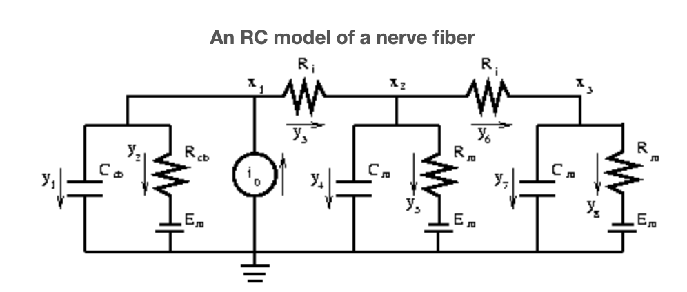
A nerve fiber's natural electrical stimulus is not direct current but rather a short burst of current, the so-called nervous impulse. In such a dynamic environment the cell's membrane behaves not only like a leaky conductor but also like a charge separator, or capacitor.
The typical value of a cell's membrane capacitance is
\[c = 1\frac{\mu F}{cm^{2}} \nonumber\]
where \(\mu F\) denotes micro-Farad. Recalling our variable conventions, the capacitance of a single compartment is
\[C_{m} = 2 \pi a \frac{l}{N} c \nonumber\]
and runs parallel to each \(R_{m}\), see Figure 1. This figure also differs from the simpler circuit from the introductory electrical modeling module in that it possesses two edges to the left of the stimuli. These edges serve to mimic that portion of the stimulus current that is shunted by the cell body. If \(A_{cb}\) denotes the surface area of the cell body, then it has
\(C_{cb} = A_{cb} c\)
\(R_{cb} = A_{cb} \rho_{m}\)
Updating the Strang Quartet
We ask now how the static Strang Quartet of the introductory electrical module should be augmented.
Updating (S1')
Regarding (S1') we proceed as before. The voltage drops are
\[e_{1} = x_{1} \nonumber\]
\[e_{2} = x_{1}-E_{m} \nonumber\]
\[e_{3} = x_{1}-x_{2} \nonumber\]
\[e_{4} = x_{2} \nonumber\]
\[e_{5} = x_{2}-E_{m} \nonumber\]
\[e_{6} = x_{2}-x_{3} \nonumber\]
\[e_{7} = x_{3} \nonumber\]
\[e_{8} = x_{3}-E_{m} \nonumber\]
and so
\[\begin{array}{ccccc} {\textbf{e} = \textbf{b}-A \textbf{x}}&{\text{where}}&{\textbf{b} = (-E_{m}) \begin{pmatrix} {0}\\ {1}\\ {0}\\ {0}\\ {1}\\ {0}\\ {0}\\ {1} \end{pmatrix}}&{\text{and}}&{A = \begin{pmatrix} {-1}&{0}&{0}\\ {-1}&{0}&{0}\\ {-1}&{1}&{0}\\ {0}&{-1}&{0}\\ {0}&{-1}&{0}\\ {0}&{-1}&{1}\\ {0}&{0}&{-1}\\ {0}&{0}&{-1} \end{pmatrix}} \end{array} \nonumber\]
Updating (S2)
To update (S2) we must now augment Ohm's law with
The current through a capacitor is proportional to the time rate of change of the potential across it.
This yields, (denoting derivative by '),
\[y_{1} = C_{cb}e_{1}′ \nonumber\]
\[y_{2} = \frac{e_{2}}{R_{cb}} \nonumber\]
\[y_{3} = \frac{e_{3}}{R_{i}} \nonumber\]
\[y_{4} = C_{m}e_{4}′ \nonumber\]
\[y_{5} = \frac{e_{5}}{R_{m}} \nonumber\]
\[y_{6} = \frac{e_{6}}{R_{i}} \nonumber\]
\[y_{7} = C_{m} e_{7}′ \nonumber\]
\[y_{8} = \frac{e_{8}}{R_{m}} \nonumber\]
or, in matrix terms,
\[\textbf{y} = G \textbf{e}+C \textbf{e}' \nonumber\]
where
\[G = \begin{pmatrix} {0}&{0}&{0}&{0}&{0}&{0}&{0}&{0}\\ {0}&{\frac{1}{R_{cb}}}&{0}&{0}&{0}&{0}&{0}&{0}\\ {0}&{0}&{\frac{1}{R_{i}}}&{0}&{0}&{0}&{0}&{0}\\ {0}&{0}&{0}&{0}&{0}&{0}&{0}&{0}\\ {0}&{0}&{0}&{0}&{\frac{1}{R_{m}}}&{0}&{0}&{0}\\ {0}&{0}&{0}&{0}&{0}&{\frac{1}{R_{i}}}&{0}&{0}\\ {0}&{0}&{0}&{0}&{0}&{0}&{0}&{0}\\ {0}&{0}&{0}&{0}&{0}&{0}&{0}&{\frac{1}{R_{m}}} \end{pmatrix} \nonumber\]
and
\[C = \begin{pmatrix} {C_{cb}}&{0}&{0}&{0}&{0}&{0}&{0}&{0}\\ {0}&{0}&{0}&{0}&{0}&{0}&{0}&{0}\\ {0}&{0}&{0}&{0}&{0}&{0}&{0}&{0}\\ {0}&{0}&{0}&{C_{m}}&{0}&{0}&{0}&{0}\\ {0}&{0}&{0}&{0}&{0}&{0}&{0}&{0}\\ {0}&{0}&{0}&{0}&{0}&{0}&{0}&{0}\\ {0}&{0}&{0}&{0}&{0}&{0}&{C_{m}}&{0}\\ {0}&{0}&{0}&{0}&{0}&{0}&{0}&{0} \end{pmatrix} \nonumber\]
are the conductance and capacitance matrices.
Updating (S3)
As Kirchhoff's Current law is insensitive to the type of device occupying an edge, step (S3) proceeds exactly as before.
\[i_{0}-y_{1}-y_{2}-y_{3} = 0 \nonumber\]
\[y_{3}-y_{4}-y_{5}-y_{6} = 0 \nonumber\]
\[y_{6}-y_{7}-y_{8} = 0 \nonumber\]
or, in matrix terms,
\[\begin{array}{ccc} {A^{T} \textbf{y} = -\textbf{f}}&{where}&{\textbf{f} = \begin{pmatrix} {i_{0}}\\ {0}\\ {0} \end{pmatrix}^{T}} \end{array} \nonumber\]
Step (S4): Assembling
Step (S4) remains one of assembling,
\[(A^{T} \textbf{y} = -\textbf{f}) \Rightarrow (A^{T} (G \textbf{e}+C \textbf{e}') = -\textbf{f}) \Rightarrow (A^{T} (G(\textbf{b}-A\textbf{x})+C (\textbf{b}'-A\textbf{x}')) = -\textbf{f}) \nonumber\]
becomes
\[A^{T}CA \textbf{x}'+A^{T}GA \textbf{x} = A^{T}G \textbf{b}+\textbf{f}+A^{T}C \textbf{b}' \nonumber\]
This is the general form of the potential equations for an RC circuit. It presumes of the user knowledge of the initial value of each of the potentials,
\[\textbf{x}(0) = X \nonumber\]
Regarding the circuit of Figure 1, and letting \(G = \frac{1}{R}\), we find
\[\begin{array}{cc} {A^{T}CA = \begin{pmatrix} {C_{cb}}&{0}&{0}\\ {0}&{C}&{0}\\ {0}&{0}&{C} \end{pmatrix}}&{A^{T}CA = \begin{pmatrix} {G_{cb}+G_{i}}&{-G_{i}}&{0}\\ {-G_{i}}&{2G_{i}+G_{m}}&{-G_{i}}\\ {0}&{-G_{i}}&{G_{i}+G_{m}} \end{pmatrix}} \end{array} \nonumber\]
\[\begin{array}{cc} {A^{T}G \textbf{b} = E_{m} \begin{pmatrix} {G_{cb}}\\ {G_{m}}\\ {G_{m}} \end{pmatrix}}&{A^{T}C \textbf{b}' = \begin{pmatrix} {0}\\ {0}\\ {0} \end{pmatrix}} \end{array} \nonumber\]
and an initial (rest) potential of
\[x_{0} = E_{m} \begin{pmatrix} {1}\\ {1}\\ {1} \end{pmatrix}^{T} \nonumber\]
Modes of Attack
We shall now outline two modes of attack on such problems. The Laplace Transform is an analytical tool that produces exact, closed-form solutions for small tractable systems and therefore offers insight into how larger systems 'should' behave. The Backward-Euler method is a technique for solving a discretized (and therefore approximate) version of Equation. It is highly flexible, easy to code, and works on problems of great size. Both the Backward-Euler and Laplace Transform methods require, at their core, the algebraic solution of a linear system of equations. In deriving these methods we shall find it more convenient to proceed from the generic system
\[\textbf{x}′ = B\textbf{x}+\textbf{g} \nonumber\]
With respect to our fiber problem
\[B = (-(A^{T}CA)^{-1}) A^{T}GA \nonumber\]
\[= \begin{pmatrix} {\frac{-(G_{cb}+G_{i})}{C_{cb}}}&{\frac{G_{i}}{C_{cb}}}&{0}\\ {\frac{G_{i}}{C_{m}}}&{\frac{-(2G_{i}+G_{m})}{C_{m}}}&{\frac{G_{i}}{C_{m}}}\\ {0}&{\frac{G_{i}}{C_{m}}}&{\frac{-(G_{i}+G_{m})}{C_{m}}} \end{pmatrix} \nonumber\]
and
\[\textbf{g} = (A^{T}CA)^{-1}(A^{T}G \textbf{b}+\textbf{f}) = \begin{pmatrix} {\frac{G_{cb}E_{m}+i_{0}}{C_{cb}}}\\ {\frac{E_{m}G_{m}}{C_{m}}}\\ {\frac{E_{m}G_{m}}{C_{m}}} \end{pmatrix} \nonumber\]