3.4: Properties of the Determinant

Learning Objectives

• Having the choice to compute the determinant of a matrix using cofactor expansion along any row or column is most useful when there are lots of what in a row or column?
• Which elementary row operation does not change the determinant of a matrix?
• Why do mathematicians rarely smile?
• T/F: When computers are used to compute the determinant of a matrix, cofactor expansion is rarely used.

In the previous section we learned how to compute the determinant. In this section we learn some of the properties of the determinant, and this will allow us to compute determinants more easily. In the next section we will see one application of determinants.

We start with a theorem that gives us more freedom when computing determinants.

Theorem \(\PageIndex{1}\)

Cofactor Expansion Along Any Row or Column

Let \(A\) be an \(n\times n\) matrix. The determinant of \(A\) can be computed using cofactor expansion along any row or column of \(A\).

We alluded to this fact way back after Example 3.3.3. We had just learned what cofactor expansion was and we practiced along the second row and down the third column. Later, we found the determinant of this matrix by computing the cofactor expansion along the first row. In all three cases, we got the number \(0\). This wasn’t a coincidence. The above theorem states that all three expansions were actually computing the determinant.

How does this help us? By giving us freedom to choose any row or column to use for the expansion, we can choose a row or column that looks “most appealing.” This usually means “it has lots of zeros.” We demonstrate this principle below.

Example \(\PageIndex{1}\)

Find the determinant of

\[A=\left[\begin{array}{cccc}{1}&{2}&{0}&{9}\\{2}&{-3}&{0}&{5}\\{7}&{2}&{3}&{8}\\{-4}&{1}&{0}&{2}\end{array}\right]. \nonumber \]

Solution

Our first reaction may well be “Oh no! Not another \(4\times 4\) determinant!” However, we can use cofactor expansion along any row or column that we choose. The third column looks great; it has lots of zeros in it. The cofactor expansion along this column is \[\begin{align}\begin{aligned} \text{det}(A) & = a_{1,3}C_{1,3} + a_{2,3}C_{2,3} + a_{3,3}C_{3,3}+a_{4,3}C_{4,3} \\ &= 0\cdot C_{1,3} + 0\cdot C_{2,3} + 3\cdot C_{3,3} + 0\cdot C_{4,3}\end{aligned}\end{align} \nonumber \]

The wonderful thing here is that three of our cofactors are multiplied by \(0\). We won’t bother computing them since they will not contribute to the determinant. Thus

\[\begin{align}\begin{aligned}\text{det}(A)&=3\cdot C_{3,3} \\ &=3\cdot (-1)^{3+3}\cdot\left|\begin{array}{ccc}{1}&{2}&{9}\\{2}&{-3}&{5}\\{-4}&{1}&{2}\end{array}\right| \\ &=3\cdot (-147)\quad\left(\begin{array}{c}{\text{we computed the determinant of the }3\times 3\text{ matrix}} \\ {\text{without showing our work; it is }-147}\end{array}\right) \\ &=-447\end{aligned}\end{align} \nonumber \]

Wow. That was a lot simpler than computing all that we did in Example 3.3.6. Of course, in that example, we didn’t really have any shortcuts that we could have employed.

Example \(\PageIndex{2}\)

Find the determinant of

\[A=\left[\begin{array}{ccccc}{1}&{2}&{3}&{4}&{5}\\{0}&{6}&{7}&{8}&{9}\\{0}&{0}&{10}&{11}&{12}\\{0}&{0}&{0}&{13}&{14} \\ {0}&{0}&{0}&{0}&{15}\end{array}\right]. \nonumber \]

Solution

At first glance, we think “I don’t want to find the determinant of a \(5\times 5\) matrix!” However, using our newfound knowledge, we see that things are not that bad. In fact, this problem is very easy.

What row or column should we choose to find the determinant along? There are two obvious choices: the first column or the last row. Both have 4 zeros in them. We choose the first column.\(^{1}\) We omit most of the cofactor expansion, since most of it is just \(0\):

\[\text{det}(A)=1\cdot (-1)^{1+1}\cdot\left|\begin{array}{cccc}{6}&{7}&{8}&{9}\\{0}&{10}&{11}&{12}\\{0}&{0}&{13}&{14}\\{0}&{0}&{0}&{15}\end{array}\right|. \nonumber \]

Similarly, this determinant is not bad to compute; we again choose to use cofactor expansion along the first column. Note: technically, this cofactor expansion is \(6\cdot(-1)^{1+1}A_{1,1}\); we are going to drop the \((-1)^{1+1}\) terms from here on out in this example (it will show up a lot...).

\[\text{det}(A)=1\cdot 6\cdot\left|\begin{array}{ccc}{10}&{11}&{12}\\{0}&{13}&{14}\\{0}&{0}&{15}\end{array}\right|. \nonumber \]

You can probably can see a trend. We’ll finish out the steps without explaining each one.

\[\begin{align}\begin{aligned}\text{det}(A)&=1\cdot 6\cdot 10\cdot\left|\begin{array}{cc}{13}&{14}\\{0}&{15}\end{array}\right| \\ &=1\cdot 6\cdot 10\cdot 13\cdot 15 \\ &=11700\end{aligned}\end{align} \nonumber \]

We see that the final determinant is the product of the diagonal entries. This works for any triangular matrix (and since diagonal matrices are triangular, it works for diagonal matrices as well). This is an important enough idea that we’ll put it into a box.

Key Idea \(\PageIndex{1}\): The Determinant of Triangular Matrices

The determinant of a triangular matrix is the product of its diagonal elements.

It is now again time to start thinking like a mathematician. Remember, mathematicians see something new and often ask “How does this relate to things I already know?” So now we ask, “If we change a matrix in some way, how is it’s determinant changed?”

The standard way that we change matrices is through elementary row operations. If we perform an elementary row operation on a matrix, how will the determinant of the new matrix compare to the determinant of the original matrix?

Let’s experiment first and then we’ll officially state what happens.

Example \(\PageIndex{3}\)

Let

\[A=\left[\begin{array}{cc}{1}&{2}\\{3}&{4}\end{array}\right]. \nonumber \]

Let \(B\) be formed from \(A\) by doing one of the following elementary row operations:

1. \(2R_{1}+R_{2}\to R_{2}\)
2. \(5R_{1}\to R_{1}\)
3. \(R_{1}\leftrightarrow R_{2}\)

Find \(\text{det}(A)\) as well as \(\text{det}(B)\) for each of the row operations above.

Solution

It is straightforward to compute \(\text{det}(A) = -2\).

Let \(B\) be formed by performing the row operation in 1) on \(A\); thus

\[B=\left[\begin{array}{cc}{1}&{2}\\{5}&{8}\end{array}\right]. \nonumber \]

It is clear that \(\text{det}(B) = -2\), the same as \(\text{det}(A)\).

Now let \(B\) be formed by performing the elementary row operation in 2) on \(A\); that is,

\[B=\left[\begin{array}{cc}{5}&{10}\\{3}&{4}\end{array}\right]. \nonumber \]

We can see that \(\text{det}(B) = -10\), which is \(5\cdot\text{det}(A)\).

Finally, let \(B\) be formed by the third row operation given; swap the two rows of \(A\). We see that

\[B=\left[\begin{array}{cc}{3}&{4}\\{1}&{2}\end{array}\right] \nonumber \]

and that \(\text{det}(B) = 2\), which is \((-1)\cdot\text{det}(A)\).

We’ve seen in the above example that there seems to be a relationship between the determinants of matrices “before and after” being changed by elementary row operations. Certainly, one example isn’t enough to base a theory on, and we have not proved anything yet. Regardless, the following theorem is true.

Theorem \(\PageIndex{2}\)

The Determinant and Elementary Row Operations

Let \(A\) be an \(n\times n\) matrix and let \(B\) be formed by performing one elementary row operation on \(A\).

1. If \(B\) is formed from \(A\) by adding a scalar multiple of one row to another, then \(\text{det}(B) = \text{det}(A)\).
2. If \(B\) is formed from \(A\) by multiplying one row of \(A\) by a scalar \(k\), then \(\text{det}(B) = k\cdot\text{det}(A)\).
3. If \(B\) is formed from \(A\) by interchanging two rows of \(A\), then \(\text{det}(B) = −\text{det}(A)\).

Let’s put this theorem to use in an example.

Example \(\PageIndex{4}\)

Let

\[A=\left[\begin{array}{ccc}{1}&{2}&{1}\\{0}&{1}&{1}\\{1}&{1}&{1}\end{array}\right]. \nonumber \]

Compute \(\text{det}(A)\), then find the determinants of the following matrices by inspection using Theorem \(\PageIndex{2}\).

\[B=\left[\begin{array}{ccc}{1}&{1}&{1}\\{1}&{2}&{1}\\{0}&{1}&{1}\end{array}\right]\quad C=\left[\begin{array}{ccc}{1}&{2}&{1}\\{0}&{1}&{1}\\{7}&{7}&{7}\end{array}\right]\quad D=\left[\begin{array}{ccc}{1}&{-1}&{-2}\\{0}&{1}&{1}\\{1}&{1}&{1}\end{array}\right] \nonumber \]

Solution

Computing \(\text{det}(A)\) by cofactor expansion down the first column or along the second row seems like the best choice, utilizing the one zero in the matrix. We can quickly confirm that \(\text{det}(A) = 1\).

To compute \(\text{det}(B)\), notice that the rows of \(A\) were rearranged to form \(B\). There are different ways to describe what happened; saying \(R_1\leftrightarrow R_2\) was followed by \(R_1\leftrightarrow R_3\) produces \(B\) from \(A\). Since there were two row swaps, \(\text{det}(B) = (-1)(-1)\text{det}(A) = \text{det}(A) = 1\).

Notice that \(C\) is formed from \(A\) by multiplying the third row by \(7\). Thus \(\text{det}(C) = 7\cdot\text{det}(A) = 7\).

It takes a little thought, but we can form \(D\) from \(A\) by the operation \(-3R_2+R_1\rightarrow R_1\). This type of elementary row operation does not change determinants, so \(\text{det}(D) = \text{det}(A)\).

Let’s continue to think like mathematicians; mathematicians tend to remember “problems” they’ve encountered in the past,\(^{2}\) and when they learn something new, in the backs of their minds they try to apply their new knowledge to solve their old problem.

What “problem” did we recently uncover? We stated in the last chapter that even computers could not compute the determinant of large matrices with cofactor expansion. How then can we compute the determinant of large matrices?

We just learned two interesting and useful facts about matrix determinants. First, the determinant of a triangular matrix is easy to compute: just multiply the diagonal elements. Secondly, we know how elementary row operations affect the determinant. Put these two ideas together: given any square matrix, we can use elementary row operations to put the matrix in triangular form,\(^{3}\) find the determinant of the new matrix (which is easy), and then adjust that number by recalling what elementary operations we performed. Let’s practice this.

Example \(\PageIndex{5}\)

Find the determinant of \(A\) by first putting \(A\) into a triangular form, where

\[A=\left[\begin{array}{ccc}{2}&{4}&{-2}\\{-1}&{-2}&{5}\\{3}&{2}&{1}\end{array}\right]. \nonumber \]

Solution

In putting \(A\) into a triangular form, we need not worry about getting leading \(1\)s, but it does tend to make our life easier as we work out a problem by hand. So let’s scale the first row by \(1/2\):

\[\frac{1}{2}R_{1}\to R_{1}\quad\left[\begin{array}{ccc}{1}&{2}&{-1}\\{-1}&{-2}&{5}\\{3}&{2}&{1}\end{array}\right]. \nonumber \]

Now let’s get \(0\)s below this leading \(1\):

\[\begin{array}{c}{R_{1}+R_{2}\to R_{2}}\\{-3R_{1}+R_{3}\to R_{3}}\end{array}\quad\left[\begin{array}{ccc}{1}&{2}&{-1}\\{0}&{0}&{4}\\{0}&{-4}&{4}\end{array}\right]. \nonumber \]

We can finish in one step; by interchanging rows \(2\) and \(3\) we’ll have our matrix in triangular form.

\[R_{2}\leftrightarrow R_{3}\quad\left[\begin{array}{ccc}{1}&{2}&{-1}\\{0}&{-4}&{4}\\{0}&{0}&{4}\end{array}\right]. \nonumber \]

Let’s name this last matrix \(B\). The determinant of \(B\) is easy to compute as it is triangular; \(\text{det}(B) = -16\). We can use this to find \(\text{det}(A)\).

Recall the steps we used to transform \(A\) into \(B\). They are:

\[\frac 12R_1 \rightarrow R_1 \nonumber \]

\[R_1 + R_2 \rightarrow R_2 \nonumber \]

\[-3R_1+R_3\rightarrow R_3 \nonumber \]

\[R_2 \leftrightarrow R_3 \nonumber \]

The first operation multiplied a row of \(A\) by \(\frac 12\). This means that the resulting matrix had a determinant that was \(\frac12\) the determinant of \(A\).

The next two operations did not affect the determinant at all. The last operation, the row swap, changed the sign. Combining these effects, we know that \[-16 = \text{det}(B)= (-1)\frac12\text{det}(A). \nonumber \]

Solving for \(\text{det}(A)\) we have that \(\text{det}(A)=32\).

In practice, we don’t need to keep track of operations where we add multiples of one row to another; they simply do not affect the determinant. Also, in practice, these steps are carried out by a computer, and computers don’t care about leading 1s. Therefore, row scaling operations are rarely used. The only things to keep track of are row swaps, and even then all we care about are the number of row swaps. An odd number of row swaps means that the original determinant has the opposite sign of the triangular form matrix; an even number of row swaps means they have the same determinant.

Let’s practice this again.

Example \(\PageIndex{6}\)

The matrix \(B\) was formed from \(A\) using the following elementary row operations, though not necessarily in this order. Find \(\text{det}(A)\).

\[B=\left[\begin{array}{ccc}{1}&{2}&{3}\\{0}&{4}&{5}\\{0}&{0}&{6}\end{array}\right] \quad\begin{array}{c}{2R_{1}\to R_{1}} \\ {\frac{1}{3}R_{3}\to R_{3}} \\ {R_{1}\leftrightarrow R_{2}} \\ {6R_{1}+R_{2}\to R_{2}}\end{array} \nonumber \]

Solution

It is easy to compute \(\text{det}(B)=24\). In looking at our list of elementary row operations, we see that only the first three have an effect on the determinant. Therefore

\[24=\text{det}(B)=2\cdot\frac{1}{3}\cdot (-1)\cdot\text{det}(A) \nonumber \]

and hence

\[\text{det}(A)=-36. \nonumber \]

In the previous example, we may have been tempted to “rebuild” \(A\) using the elementary row operations and then computing the determinant. This can be done, but in general it is a bad idea; it takes too much work and it is too easy to make a mistake.

Let’s think some more like a mathematician. How does the determinant work with other matrix operations that we know? Specifically, how does the determinant interact with matrix addition, scalar multiplication, matrix multiplication, the transpose and the trace? We’ll again do an example to get an idea of what is going on, then give a theorem to state what is true.

Example \(\PageIndex{7}\)

Let

\[A=\left[\begin{array}{cc}{1}&{2}\\{3}&{4}\end{array}\right]\quad\text{and}\quad B=\left[\begin{array}{cc}{2}&{1}\\{3}&{5}\end{array}\right]. \nonumber \]

Find the determinants of the matrices \(A\), \(B\), \(A + B\), \(3A\), \(AB\), \(A^{T}\), \(A^{−1}\), and compare the determinant of these matrices to their trace.

Solution

We can quickly compute that \(\text{det}(A) = -2\) and that \(\text{det}(B) = 7\).

\[\begin{align}\begin{aligned}\text{det}(A-B)&=\text{det}\left(\left[\begin{array}{cc}{1}&{2}\\{3}&{4}\end{array}\right]-\left[\begin{array}{cc}{2}&{1}\\{3}&{5}\end{array}\right]\right) \\ &=\left|\begin{array}{cc}{-1}&{1}\\{0}&{-1}\end{array}\right| \\ &=1\end{aligned}\end{align} \nonumber \]

It’s tough to find a connection between \(\text{det}(A-b)\), \(\text{det}(A)\) and \(\text{det}(B)\).

\[\begin{align}\begin{aligned}\text{det}(3A)&=\left|\begin{array}{cc}{3}&{6}\\{9}&{12}\end{array}\right| \\ &=-18\end{aligned}\end{align} \nonumber \]

We can figure this one out; multiplying one row of \(A\) by \(3\) increases the determinant by a factor of \(3\); doing it again (and hence multiplying both rows by \(3\)) increases the determinant again by a factor of \(3\). Therefore \(\text{det}(3A)=3\cdot 3\cdot\text{det}(A)\), or \(3^{2}\cdot A\).

\[\begin{align}\begin{aligned}\text{det}(AB)&=\text{det}\left(\left[\begin{array}{cc}{1}&{2}\\{3}&{4}\end{array}\right]\left[\begin{array}{cc}{2}&{1}\\{3}&{5}\end{array}\right]\right) \\ &=\left|\begin{array}{cc}{8}&{11}\\{18}&{23}\end{array}\right| \\ &=-14\end{aligned}\end{align} \nonumber \]

This one seems clear; \(\text{det}(AB)=\text{det}(A)\text{det}(B)\).

\[\begin{align}\begin{aligned}\text{det}(A^{T})&=\left|\begin{array}{cc}{1}&{3}\\{2}&{4}\end{array}\right| \\ &=-2\end{aligned}\end{align} \nonumber \]

Obviously \(\text{det}(A^{T})=\text{det}(A)\); is this always going to be the case? If we think about it, we can see that the cofactor expansion along the first row of \(A\) will give us the same result as the cofactor expansion along the first column of \(A\).\(^{4}\)

\[\begin{align}\begin{aligned}\text{det}(A^{-1})&=\left|\begin{array}{cc}{-2}&{1}\\{3/2}&{-1/2}\end{array}\right| \\ &=1-3/2 \\ &=-1/2\end{aligned}\end{align} \nonumber \]

It seems as though

\[\text{det}(A^{-1})=\frac{1}{\text{det}(A)}. \nonumber \]

We end by remarking that there seems to be no connection whatsoever between the trace of a matrix and its determinant. We leave it to the reader to compute the trace for some of the above matrices and confirm this statement.

We now state a theorem which will confirm our conjectures from the previous example.

Theorem \(\PageIndex{3}\)

Determinant Properties

Let \(A\) and \(B\) be \(n\times n\) matrices and let \(k\) be a scaler. The following are true:

1. \(\text{det}(kA)=k^{n}\cdot\text{det}(A)\)
2. \(\text{det}(A^{T})=\text{det}(A)\)
3. \(\text{det}(AB)=\text{det}(A)\text{det}(B)\)
4. If \(A\) is invertible, then
   \[\text{det}(A^{-1})=\frac{1}{\text{det}(A)}.\nonumber \]
5. A matrix \(A\) is invertible if and only if \(\text{det}(A)\neq 0\).

This last statement of the above theorem is significant: what happens if \(\text{det}(A) = 0\)? It seems that \(\text{det}(A^{-1})="1/0"\), which is undefined. There actually isn’t a problem here; it turns out that if \(\text{det}(A)=0\), then \(A\) is not invertible (hence part 5 of Theorem \(\PageIndex{3}\)). This allows us to add on to our Invertible Matrix Theorem.

Theorem \(\PageIndex{4}\)

Invertible Matrix Theorem

Let \(A\) be an \(n\times n\) matrix. The following statements are equivalent.

1. \(A\) is invertible.
2. \(\text{det}(A)\neq 0\).

This new addition to the Invertible Matrix Theorem is very useful; we’ll refer back to it in Chapter 4 when we discuss eigenvalues.

We end this section with a shortcut for computing the determinants of \(3\times 3\) matrices. Consider the matrix \(A\):

\[\left[\begin{array}{ccc}{1}&{2}&{3}\\{4}&{5}&{6}\\{7}&{8}&{9}\end{array}\right]. \nonumber \]

We can compute its determinant using cofactor expansion as we did in Example 3.3.4. Once one becomes proficient at this method, computing the determinant of a \(3\times3\) isn’t all that hard. A method many find easier, though, starts with rewriting the matrix without the brackets, and repeating the first and second columns at the end as shown below. \[\begin{array}{ccccc} 1&2&3&1&2 \\ 4 & 5 & 6&4&5\\7&8&9&7&8\end{array} \nonumber \]

In this \(3\times 5\) array of numbers, there are 3 full “upper left to lower right” diagonals, and 3 full “upper right to lower left” diagonals, as shown below with the arrows.

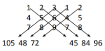
The numbers that appear at the ends of each of the arrows are computed by multiplying the numbers found along the arrows. For instance, the \(105\) comes from multiplying \(3\cdot5\cdot7=105\). The determinant is found by adding the numbers on the right, and subtracting the sum of the numbers on the left. That is, \[\text{det}(A) = (45+84+96) - (105+48+72) = 0. \nonumber \]

To help remind ourselves of this shortcut, we’ll make it into a Key Idea.

Key Idea \(\PageIndex{2}\): \(3\times 3\) Determinant Shortcut

Let \(A\) be a \(3\times 3\) matrix. Create a \(3\times 5\) array by repeating the first \(2\) columns and consider the products of the \(3\) “right hand” diagonals and \(3\) “left hand” diagonals as shown previously. Then

\[\begin{align}\begin{aligned}\text{det}(A)&=\text{"(the sum of the right hand numbers)} \\ & -\text{(the sum of the left hand numbers)".}\end{aligned}\end{align} \nonumber \]

We’ll practice once more in the context of an example.

Example \(\PageIndex{8}\)

Find the determinant of \(A\) using the previously described shortcut, where

\[A=\left[\begin{array}{ccc}{1}&{3}&{9}\\{-2}&{3}&{4}\\{-5}&{7}&{2}\end{array}\right]. \nonumber \]

Solution

Rewriting the first \(2\) columns, drawing the proper diagonals, and multiplying, we get:

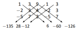
Summing the numbers on the right and subtracting the sum of the numbers on the left, we get \[\text{det}(A) = (6-60-126) - ( -135+28-12) = -61. \nonumber \]

In the next section we’ll see how the determinant can be used to solve systems of linear equations.

Footnotes

[1] We do not choose this because it is the better choice; both options are good. We simply had to make a choice.

[2] which is why mathematicians rarely smile: they are remembering their problems

[3] or echelon form

[4] This can be a bit tricky to think out in your head. Try it with a 3\(\times 3\) matrix \(A\) and see how it works. All the \(2\times 2\) submatrices that are created in \(A^{T}\) are the transpose of those found in \(A\); this doesn’t matter since it is easy to see that the determinant isn’t affected by the transpose in a \(2\times 2\) matrix.