
1.2: Row Reduction
- Page ID
- 70183

\( \( \def\d{\displaystyle}\)
\( \newcommand{\f}[1]{\mathfrak #1}\)
\( \newcommand{\s}[1]{\mathscr #1}\)
\(\def\R{\mathbf R}\)
\( \def\C{\mathbf C}\)
\( \let\mathbb=\mathbf\)
\( \let\oldvec=\vec\)
\( \let\vec=\spalignvector\)
\( \let\mat=\spalignmat\)
\( \let\amat=\spalignaumat\)
\( \let\hmat=\spalignaugmathalf\)
\( \let\syseq=\spalignsys\)
\( \let\epsilon=\varepsilon\)
\( \def\Span{\operatorname{Span}}\)
\( \def\Nul{\operatorname{Nul}}\)
\( \def\Col{\operatorname{Col}}\)
\( \def\Row{\operatorname{Row}}\)
\( \def\rank{\operatorname{rank}}\)
\( \def\nullity{\operatorname{nullity}}\)
\( \def\Id{\operatorname{Id}}\)
\( \def\Tr{\operatorname{Tr}}\)
\( \def\adj{\operatorname{adj}}\)
\( \def\Re{\operatorname{Re}}\)
\( \def\Im{\operatorname{Im}}\)
\( \def\dist{\operatorname{dist}}\)
\( \def\refl{\operatorname{ref}}\)
\( \def\inv{^{-1}}\)
\( \let\To=\longrightarrow\)
\( \def\rref{\;\xrightarrow{\text{RREF}}\;}\)
\( \def\matrow#1{\text{---}\,#1\,\text{---}}\)
\( \def\vol{\operatorname{vol}}\)
\( \def\sptxt#1{\quad\text{ #1 }\quad}\)
\( \let\bar=\overline\)
\( \let\hat=\widehat\)
\(\( \def\cB
Callstack:
    at (Template:MathJazMargalit), /content/body/div/p[4]/span, line 1, column 1
    at template()
    at (Bookshelves/Linear_Algebra/Interactive_Linear_Algebra_(Margalit_and_Rabinoff)/01:_Systems_of_Linear_Equations-_Algebra/1.02:_Row_Reduction), /content/body/p[1]/span, line 1, column 25
\(\newcommand{\leading}[1]{\color{red}#1}\)
\(\newcommand{\setof}[1]{\left\{#1\right\}}\)
- Learn to replace a system of linear equations by an augmented matrix.
- Learn how the elimination method corresponds to performing row operations on an augmented matrix.
- Understand when a matrix is in (reduced) row echelon form.
- Learn which row reduced matrices come from inconsistent linear systems.
- Recipe: the row reduction algorithm.
- Vocabulary words: row operation, row equivalence, matrix, augmented matrix, pivot, (reduced) row echelon form.
In this section, we will present an algorithm for “solving” a system of linear equations.
The Elimination Method
We will solve systems of linear equations algebraically using the elimination method. In other words, we will combine the equations in various ways to try to eliminate as many variables as possible from each equation. There are three valid operations we can perform on our system of equations:
- Scaling: we can multiply both sides of an equation by a nonzero number.
\[\left\{\begin{array}{rrrrrrr}x &+& 2y &+& 3z &=& 6\\ 2x &-& 3y &+& 2z &=& 14\\ 3x &+& y &-& z &=& -2\end{array}\right. \quad\xrightarrow{\text{multiply 1st by $-3$}}\quad \left\{\begin{array}{rrrrrrr} -3x &-& 6y &-& 9z &=& -18\\ 2x &-& 3y &+& 2z &=& 14\\ 3x &+& y &-& z &=& -2\end{array}\right. \nonumber \] - Replacement: we can add a multiple of one equation to another, replacing the second equation with the result.
\[\left\{\begin{array}{rrrrrrr}x &+& 2y &+& 3z &=& 6\\ 2x &-& 3y &+& 2z &=& 14\\ 3x &+& y &-& z &=& -2 \end{array}\right. \quad\xrightarrow{\text{2nd ${}={}$ 2nd$-2\times$1st}}\quad \left\{\begin{array}{rrrrrrr} x &+& 2y &+& 3z &=& 6\\ {}&{}& -7y &-& 4z &=& 2\\ 3x &+& y &-& z &=& -2\end{array}\right.\nonumber\] - Swap: we can swap two equations.
\[\left\{\begin{array}{rrrrrrr}x &+& 2y &+& 3z &=& 6\\ 2x &-& 3y &+& 2z &=& 14\\ 3x &+& y &-& z &=& -2 \end{array}\right. \quad\xrightarrow{\text{3rd $\longleftrightarrow$ 1st}}\quad \left\{\begin{array}{rrrrrrr} 3x &+& y &-& z &=& -2\\ 2x &-& 3y &+& 2z &=& 14\\ x &+& 2y &+& 3z &=& 6\end{array}\right.\nonumber\]
Solve Equation (1.1.1) using the elimination method.
Solution
\[\begin{aligned} \left\{\begin{array}{rrrrrrr} x &+& 2y &+& 3z &=& 6\\ 2x &-& 3y &+& 2z &=& 14\\ 3x &+& y &-& z &=& -2\end{array}\right. \quad\xrightarrow{\text{2nd ${}={}$ 2nd$-2\times$1st}}\quad & \left\{\begin{array}{rrrrrrr}x &+& 2y &+& 3z &=& 6\\ {}&{}& -7y &-& 4z &=& 2\\ 3x &+& y &-& z &=& -2 \end{array}\right. \\ {} \quad\xrightarrow{\text{3rd ${}={}$ 3rd$-3\times$1st}}\quad& \left\{\begin{array}{rrrrrrr} x &+& 2y &+& 3z &=& 6 \\ {}&{}& -7y &-& 4z &=& 2\\ {}&{}& -5y &-& 10z &=& -20 \end{array}\right. \\ {} \quad\xrightarrow{\text{2nd $\longleftrightarrow$ 3rd}}\quad & \left\{\begin{array}{rrrrrrr} x &+& 2y &+& 3z &=& 6\\ {}&{}& -5y &-& 10z &=& -20 \\ {}&{}& -7y &-& 4z &=& 2\end{array}\right. \\ {} \quad\xrightarrow{\text{divide 2nd by $-5$}}\quad & \left\{\begin{array}{rrrrrrr} x &+& 2y &+& 3z &=& 6 \\ {}&{}& y &+& 2z &=& 4\\ {}&{}& -7y &-& 4z &=& 2 \end{array}\right. \\ {} \quad\xrightarrow{\text{3rd ${}={}$ 3rd$+7\times$2nd}}\quad & \left\{\begin{array}{rrrrrrr} x &+& 2y &+& 3z &=& 6\\ {}&{}&y &+& 2z &=& 4 \\ {}&{}&{}&{}&10z &=& 30 \end{array}\right.\end{aligned}\]
At this point we’ve eliminated both \(x\) and \(y\) from the third equation, and we can solve \(10z=30\) to get \(z=3\). Substituting for \(z\) in the second equation gives \(y+2\cdot3=4\text{,}\) or \(y=-2\). Substituting for \(y\) and \(z\) in the first equation gives \(x + 2\cdot(-2) + 3\cdot3 = 6\text{,}\) or \(x=3\). Thus the only solution is \((x,y,z)=(1,-2,3)\).
We can check that our solution is correct by substituting \((x,y,z)=(1,-2,3)\) into the original equation:
\[\left\{\begin{array}{rrrrrrr} x &+& 2y &+& 3z &=& 6 \\ 2x &-& 3y &+& 2z &=& 14 \\ 3x &+& y &-& z &=& -2 \end{array}\right. \quad\xrightarrow{\text{substitute}}\quad \left\{\begin{array}{rrrrrrr} 1 &2&\cdot(-2) &+& 3\cdot 3 &=& 6 \\ 2\cdot 1 &-& 3\cdot(-2) &+& 2\cdot 3 &=& 14 \\ 3\cdot 1 &+& (-2) &-& 3 &=& -2 \end{array}\right. \nonumber\]
Augmented Matrices and Row Operations
Solving equations by elimination requires writing the variables \(x,y,z\) and the equals sign \(=\) over and over again, merely as placeholders: all that is changing in the equations is the coefficient numbers. We can make our life easier by extracting only the numbers, and putting them in a box:
\[\left\{\begin{array}{rrrrrrr} x &+& 2y &+& 3z &=& 6\\ 2x &-& 3y &+& 2z& =& 14\\ 3x &+& y &-& z &=& -2\end{array}\right. \quad\xrightarrow{\text{becomes}}\quad \left(\begin{array}{ccc|c} 1&2&3&6 \\ 2&-3&2&14 \\ 3&1&-1&-2 \end{array}\right).\nonumber\]
This is called an augmented matrix. The word “augmented” refers to the vertical line, which we draw to remind ourselves where the equals sign belongs; a matrix is a grid of numbers without the vertical line. In this notation, our three valid ways of manipulating our equations become row operations:
- Scaling: multiply all entries in a row by a nonzero number.
\[\left(\begin{array}{ccc|c} 1& 2& 3& 6&\\ 2& -3& 2& 14\\ 3& 1& -1& -2\end{array}\right) \quad\xrightarrow{R_1 = R_1 \times -3}\quad \left(\begin{array}{ccc|c} -3 &-6 &-9 &-18\\ 2& -3& 2& 14\\ 3& 1& -1& -2\end{array}\right)\nonumber\]
Here the notation \(R_1\) simply means “the first row”, and likewise for \(R_2,R_3,\) etc. - Replacement: add a multiple of one row to another, replacing the second row with the result.
\[\left(\begin{array}{ccc|c}1 &2& 3& 6\\ 2& -3& 2& 14\\ 3& 1& -1& -2\end{array}\right) \quad\xrightarrow{R_2 = R_2 -2\times R_1}\quad \left(\begin{array}{ccc|c} 1 &2 &3 &6 \\ 0& -7& -4& 2\\ 3& 1& -1& -2\end{array}\right)\nonumber\] - Swap: interchange two rows.
\[\left(\begin{array}{ccc|c} 1 &2 &3 &6 \\ 2& -3& 2& 14\\ 3& 1& -1& -2\end{array}\right) \quad\xrightarrow{R_1 \longleftrightarrow R_3}\quad \left(\begin{array}{ccc|c} 3 &1 &-1& -2\\ 2& -3& 2& 14\\ 1& 2& 3& 6\end{array}\right)\nonumber\]
When we wrote our row operations above we used expressions like \(R_2 = R_2 - 2 \times R_1\). Of course this does not mean that the second row is equal to the second row minus twice the first row. Instead it means that we are replacing the second row with the second row minus twice the first row. This kind of syntax is used frequently in computer programming when we want to change the value of a variable.
Solve Equation (1.1.1) using row operations.
Solution
We start by forming an augmented matrix:
\[\left\{\begin{array}{rrrrrrr} x&+&2y&+&3x&=& 6\\ 2x&-&3y&+&2z&=&14 \\ 3x&+&y&-&z&=&-2 \end{array}\right. \quad\xrightarrow{\text{becomes}}\quad \left(\begin{array}{ccc|c}1&2&3&6\\2&-3&2&14\\3&1&-1&-2\end{array}\right).\nonumber \]
Eliminating a variable from an equation means producing a zero to the left of the line in an augmented matrix. First we produce zeros in the first column (i.e. we eliminate \(x\)) by subtracting multiples of the first row.
\[\begin{aligned} \left(\begin{array}{ccc|c} 1 &2 &3& 6\\ 2& -3& 2& 14\\ 3& 1& -1& -2\end{array}\right) & \quad\xrightarrow{R_2=R_2-2R_1}\quad \left(\begin{array}{ccc|c} 1 &2 &3& 6\\ \color{red}{0}& -7& -4& 2\\ 3& 1& -1& -2\end{array}\right) \\ & \quad\xrightarrow{R_3=R_3-3R_1}\quad \left(\begin{array}{ccc|c} 1 &2& 3& 6\\ 0& -7& -4& 2\\ \color{red}{0}& -5& -10& -20\end{array}\right) \end{aligned}\]
This was made much easier by the fact that the top-left entry is equal to \(1\text{,}\) so we can simply multiply the first row by the number below and subtract. In order to eliminate \(y\) in the same way, we would like to produce a \(1\) in the second column. We could divide the second row by \(-7\text{,}\) but this would produce fractions; instead, let’s divide the third by \(-5\).
\[\begin{aligned} \left(\begin{array}{ccc|c} 1 &2& 3& 6\\ 0& -7& -4& 2\\ 0& -5& -10& -20 \end{array}\right) \quad\xrightarrow{R_3=R_3\div-5}\quad & \left(\begin{array}{ccc|c} 1 &2& 3& 6\\ 0 &-7& -4& 2\\ 0& \color{red}{1}& 2& 4\end{array}\right) \\ {}\quad\xrightarrow{R_2\longleftrightarrow R_3}\quad & \left(\begin{array}{ccc|c} 1 &2& 3& 6\\ 0& 1& 2& 4 \\ 0& -7& -4& 2\end{array}\right) \\ {}\quad\xrightarrow{R_3 = R_3+7R_2}\quad & \left(\begin{array}{ccc|c} 1 &2& 3& 6\\ 0& 1& 2& 4\\ 0& \color{red}{0} & 10& 30 \end{array}\right) \\ {}\quad\xrightarrow{R_3 = R_3\div 10}\quad & \left(\begin{array}{ccc|c}1 &2& 3& 6\\ 0& 1& 2& 4 \\ 0& 0& \color{red}{1}& 3\end{array}\right)\end{aligned}\]
We swapped the second and third row just to keep things orderly. Now we translate this augmented matrix back into a system of equations:
\[\left(\begin{array}{ccc|c} 1 &2& 3& 6\\ 0& 1& 2& 4\\ 0& 0& 1& 3\end{array}\right) \quad\xrightarrow{\text{becomes}}\quad \left\{\begin{array}{rrrrrrr} x &+& 2y &+& 3z &=& 6 \\ {}&{}& y &+& 2z &=& 4 \\ {}&{}&{}&{}&z &=& 3\end{array}\right.\nonumber \]
Hence \(z=3\text{;}\) back-substituting as in Example \(\PageIndex{1}\) gives \((x,y,z)=(1,-2,3)\).
The process of doing row operations to a matrix does not change the solution set of the corresponding linear equations!
Indeed, the whole point of doing these operations is to solve the equations using the elimination method.
Two matrices are called row equivalent if one can be obtained from the other by doing some number of row operations.
So the linear equations of row-equivalent matrices have the same solution set.
Solve the following system of equations using row operations:
\[\left\{\begin{array}{rrrrr} x &+& y& =& 2\\ 3x &+& 4y &=& 5\\ 4x &+ &5y &=& 9\end{array}\right. \nonumber\]
Solution
First we put our system of equations into an augmented matrix.
\[\left\{\begin{array}{rrrrr} x &+& y &=& 2\\ 3x &+& 4y &=& 5\\ 4x &+& 5y &=& 9\end{array}\right. \quad\xrightarrow{\text{augmented matrix}}\quad \left(\begin{array}{cc|c} 1 &1& 2\\ 3 &4& 5\\ 4& 5& 9\end{array}\right) \nonumber\]
We clear the entries below the top-left using row replacement.
\[\begin{aligned}\left(\begin{array}{cc|c} 1 &1& 2\\ 3& 4& 5\\ 4& 5& 9\end{array}\right) \quad\xrightarrow{R_2=R_2-3R_1}\quad & \left(\begin{array}{cc|c} 1 &1& 2\\ \color{red}{0} & 1& -1\\ 4& 5& 9\end{array}\right) \\ {} \quad\xrightarrow{R_3=R_3-4R_1}\quad & \left(\begin{array}{cc|c} 1 &1& 2\\ 0& 1& -1\\ \color{red}{0}& 1& 1\end{array}\right)\end{aligned}\]
Now we clear the second entry from the last row.
\[\left(\begin{array}{cc|c} 1 &1& 2\\ 0& 1& -1\\ 0 &1& 1\end{array}\right) \quad\xrightarrow{R_3=R_3-R_2}\quad \left(\begin{array}{cc|c} 1 &1& 2\\ 0& 1& -1\\ 0& \color{red}{0}& 2\end{array}\right) \nonumber \]
This translates back into the system of equations
\[\left\{\begin{array}{rrrrr} x &+& y &=& 2\\ {}&{}& y& =& -1 \\ {}&{}& 0& =& 2. \end{array}\right. \nonumber\]
Our original system has the same solution set as this system. But this system has no solutions: there are no values of \(x,y\) making the third equation true! We conclude that our original equation was inconsistent.
Echelon Forms
In the previous Subsection The Elimination Method we saw how to translate a system of linear equations into an augmented matrix. We want to find an algorithm for “solving” such an augmented matrix. First we must decide what it means for an augmented matrix to be “solved”.
A matrix is in row echelon form if:
- All zero rows are at the bottom.
- The first nonzero entry of a row is to the right of the first nonzero entry of the row above.
- Below the first nonzero entry of a row, all entries are zero.
Here is a picture of a matrix in row echelon form:
\[\left(\begin{array}{ccccc} \color{red}{\boxed{\star}} &\star &\star &\star &\star \\ 0&\color{red}{\boxed{\star}} & \star &\star &\star \\ 0&0&0&\color{red}{\boxed{\star}} &\star \\ 0&0&0&0&0 \end{array}\right) \qquad \begin{aligned} \star &= \text{any number} \\ \color{red}\boxed\star &= \text{any nonzero number} \end{aligned} \nonumber \]
A pivot is the first nonzero entry of a row of a matrix in row echelon form.
A matrix in row-echelon form is generally easy to solve using back-substitution. For example,
\[\left(\begin{array}{ccc|c} 1 &2& 3& 6\\ 0& 1& 2& 4 \\ 0& 0& 10& 30 \end{array}\right) \quad\xrightarrow{\text{becomes}}\quad \left\{\begin{array}{rrrrrrr} x &+& 2y &+& 3z &=& 6 \\ {}&{}& y &+& 2z& =& 4 \\ {}&{}&{}&{}& 10z &=& 30. \end{array}\right. \nonumber\]
We immediately see that \(z=3\text{,}\) which implies \(y = 4-2\cdot 3 = -2\) and \(x = 6 - 2(-2) - 3\cdot 3 = 1.\) See Example \(\PageIndex{3}\).
A matrix is in reduced row echelon form if it is in row echelon form, and in addition:
- Each pivot is equal to 1.
- Each pivot is the only nonzero entry in its column.
Here is a picture of a matrix in reduced row echelon form:
\[\left(\begin{array}{ccccc} \color{red}{1} &0&\star &0&\star \\ 0&\color{red}{1} &\star &0 &\star \\ 0&0&0&\color{red}{1}&\star \\ 0&0&0&0&0\end{array}\right) \qquad \begin{aligned} \star &= \text{any number} \\ \color{red}1 &= \text{pivot} \end{aligned} \nonumber\]
A matrix in reduced row echelon form is in some sense completely solved. For example,
\[\left(\begin{array}{ccc|c} 1 &0& 0& 1\\ 0& 1& 0& -2\\ 0& 0& 1& 3\end{array}\right) \quad\xrightarrow{\text{becomes}}\quad \left\{\begin{array}{rrr} x &=& 1\\ y &=& -2 \\ z &=& 3.\end{array}\right. \nonumber \]
The following matrices are in reduced row echelon form:
\[\left(\begin{array}{ccc}1&0&2 \\ 0&1&-1\end{array}\right)\qquad \left(\begin{array}{cccc}0&1&8&0\end{array}\right) \qquad \left(\begin{array}{cc|c} 1&17&0\\0&0&1\end{array}\right)\qquad\left(\begin{array}{ccc}0&0&0\\0&0&0\end{array}\right).\nonumber\]
The following matrices are in row echelon form but not reduced row echelon form:
\[\left(\begin{array}{cc}2&1\\0&1\end{array}\right)\qquad \left(\begin{array}{ccc|c} 2&7&1&4 \\ 0&0&2&1 \\ 0&0&0&3\end{array}\right)\qquad \left(\begin{array}{ccc}1&17&0\\0&1&1\end{array}\right) \qquad \left(\begin{array}{ccc}2&1&3\\0&0&0\end{array}\right).\nonumber\]
The following matrices are not in echelon form:
\[\left(\begin{array}{ccc|c} 2&7&1&4\\0&0&2&1\\0&0&1&3 \end{array}\right)\qquad\left(\begin{array}{cc|c}0&17&0\\0&2&1\end{array}\right)\qquad\left(\begin{array}{cc}2&1\\2&1\end{array}\right) \qquad \left(\begin{array}{c}0\\1\\0\\0\end{array}\right).\nonumber\]
When deciding if an augmented matrix is in (reduced) row echelon form, there is nothing special about the augmented column(s). Just ignore the vertical line.
If an augmented matrix is in reduced row echelon form, the corresponding linear system is viewed as solved. We will see below why this is the case, and we will show that any matrix can be put into reduced row echelon form using only row operations.
Consider the following system of equations:
\[\left\{\begin{array}{rrrrr}x &-& y &=& 0\\ x &+& y &=& 2.\end{array}\right.\nonumber\]
We can visualize this system as a pair of lines in \(\mathbb{R}^2\) (red and blue, respectively, in the picture below) that intersect at the point \((1,1)\). If we subtract the first equation from the second, we obtain the equation \(2y=2\text{,}\) or \(y=1\). This results in the system of equations:
\[\left\{\begin{array}{rrrrr}x &-& y &=& 0 \\ {}&{} &y &=& 1.\end{array}\right.\nonumber\]
In terms of row operations on matrices, we can write this as:
\[\begin{aligned} \left(\begin{array}{cc|c} 1&-1&0 \\ 1&1&2\end{array}\right) \quad\xrightarrow{R_2=R_2-R_1}\quad & \left(\begin{array}{cc|c} 1&-1&0 \\ 0&2&2\end{array}\right) \\ {} \quad\xrightarrow{R_2=\frac{1}{2}R_2}\quad & \left(\begin{array}{cc|c} 1&-1&0\\0&1&1\end{array}\right)\end{aligned}\]
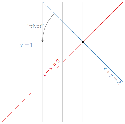
Figure \(\PageIndex{1}\)
What has happened geometrically is that the original blue line has been replaced with the new blue line \(y=1\). We can think of the blue line as rotating, or pivoting, around the solution \((1,1)\). We used the pivot position in the matrix in order to make the blue line pivot like this. This is one possible explanation for the terminology “pivot”.
The Row Reduction Algorithm
Every matrix is row equivalent to one and only one matrix in reduced row echelon form.
We will give an algorithm, called row reduction or Gaussian elimination, which demonstrates that every matrix is row equivalent to at least one matrix in reduced row echelon form.
The uniqueness statement is interesting—it means that, no matter how you row reduce, you always get the same matrix in reduced row echelon form.
This assumes, of course, that you only do the three legal row operations, and you don’t make any arithmetic errors.
We will not prove uniqueness, but maybe you can!
- Step 1a: Swap the 1st row with a lower one so a leftmost nonzero entry is in the 1st row (if necessary).
- Step 1b: Scale the 1st row so that its first nonzero entry is equal to 1.
- Step 1c: Use row replacement so all entries below this 1 are 0.
- Step 2a: Swap the 2nd row with a lower one so that the leftmost nonzero entry is in the 2nd row.
- Step 2b: Scale the 2nd row so that its first nonzero entry is equal to 1.
- Step 2c: Use row replacement so all entries below this 1 are 0.
- Step 3a: Swap the 3rd row with a lower one so that the leftmost nonzero entry is in the 3rd row.
- etc.
- Last Step: Use row replacement to clear all entries above the pivots, starting with the last pivot.
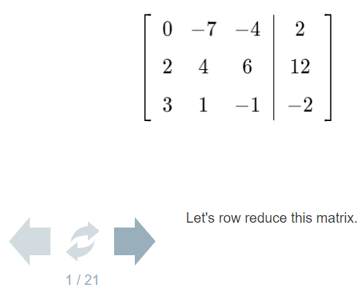
Row reduce this matrix:
\[\left(\begin{array}{ccc|c} 0&-7&-4&2 \\ 2&4&6&12\\ 3&1&-1&-2\end{array}\right).\nonumber\]
Solution
The reduced row echelon form of the matrix is
\[\left(\begin{array}{ccc|c}1&0&0&1 \\ 0&1&0&-2\\0&0&1&3\end{array}\right) \quad\xrightarrow{\text{translates to}}\quad \left\{\begin{array}{rrrrrrr} x&{}&{}&{}&{}&=&1 \\ {}&{}&y&{}&{}&=&-2 \\ {}&{}&{}&{}&z&=&3.\end{array}\right.\nonumber\]
The reduced row echelon form of the matrix tells us that the only solution is \((x,y,z) = (1,-2,3).\)
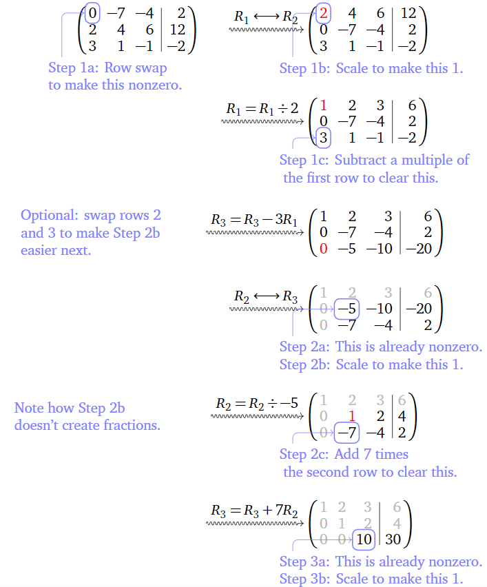
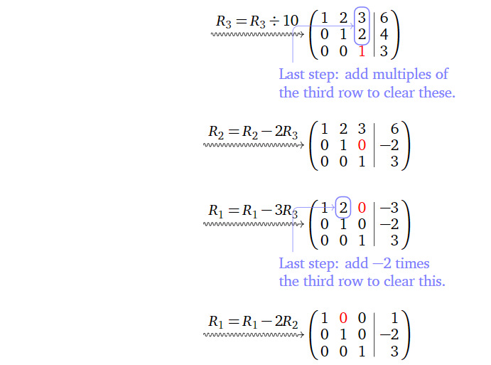
Here is the row reduction algorithm, summarized in pictures.
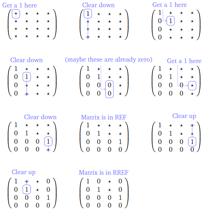
Figure \(\PageIndex{3}\)
It will be very important to know where are the pivots of a matrix after row reducing; this is the reason for the following piece of terminology.
A pivot position of a matrix is an entry that is a pivot of a row echelon form of that matrix.
A pivot column of a matrix is a column that contains a pivot position.
Find the pivot positions and pivot columns of this matrix
\[A=\left(\begin{array}{ccc|c} 0 &-7& -4& 2\\ 2& 4& 6& 12 \\ 3& 1& -1& -2\end{array}\right).\nonumber\]
Solution
We saw in Example \(\PageIndex{5}\) that a row echelon form of the matrix is
\[\left(\begin{array}{ccc|c} 1 &2& 3& 6\\ 0& 1& 2& 4\\ 0& 0& 10& 30\end{array}\right).\nonumber\]
The pivot positions of \(A\) are the entries that become pivots in a row echelon form; they are marked in red below:
\[\left(\begin{array}{ccc|c}\color{red}{0}&-7&-4&2 \\ 2&\color{red}{4}&6&12 \\ 3&1&\color{red}{-1}&-2\end{array}\right).\nonumber\]
The first, second, and third columns are pivot columns.
Solve the linear system
\[\left\{\begin{array}{rrrrr}2x &+& 10y &=& -1 \\ 3x &+& 15y &=& 2\end{array}\right. \nonumber \]
using row reduction.
Solution
\[\begin{aligned} \left(\begin{array}{cc|c} 2&10&-1 \\ 3&15&2 \end{array}\right) \quad\xrightarrow{R_1=R_1\div 2}\quad & \left(\begin{array}{cc|c} \color{red}{1}&5&{-\frac{1}{2}} \\ 3&15&2 \end{array}\right) &&\color{blue}{\text{(Step 1b)}} \\ {} \quad\xrightarrow{R_2=R_2-3R_1}\quad & \left(\begin{array}{cc|c} 1&5&{-\frac{1}{2}} \\ \color{red}{0} &0&{\frac{7}{2}} \end{array}\right) &&\color{blue}{\text{(Step 1c)}} \\ {}\quad\xrightarrow{R_2=R_2\times\frac 27}\quad & \left(\begin{array}{cc|c} 1&5&{-\frac{1}{2}} \\ 0&0&\color{red}{1} \end{array}\right) &&\color{blue}{\text{(Step 2b)}} \\ {} \quad\xrightarrow{R_1=R_1+\frac 12R_2}\quad & \left(\begin{array}{cc|c} 1&5&\color{red}{0} \\ 0&0&1\end{array}\right) &&\color{blue}{\text{(Step 2c)}}\end{aligned}\]
This row reduced matrix corresponds to the inconsistent system
\[\left\{\begin{array}{rrrrr} x &+& 5y &=& 0\\ {}&{}&0& =& 1. \end{array}\right. \nonumber \]
In the above example, we saw how to recognize the reduced row echelon form of an inconsistent system.
An augmented matrix corresponds to an inconsistent system of equations if and only if the last column (i.e., the augmented column) is a pivot column.
In other words, the row reduced matrix of an inconsistent system looks like this:
\[\left(\begin{array}{cccc|c} 1&0&\star &\star &\color{red}{0} \\ 0&1&\star &\star &\color{red}{0}\\ 0&0&0&0&\color{red}{1}\end{array}\right)\nonumber\]
We have discussed two classes of matrices so far:
- When the reduced row echelon form of a matrix has a pivot in every non-augmented column, then it corresponds to a system with a unique solution:
\[\left(\begin{array}{ccc|c} 1 &0& 0& 1\\ 0& 1& 0& -2\\ 0& 0& 1& 3\end{array}\right) \quad\xrightarrow{\text{translates to}}\quad \left\{\begin{array}{rrrrrrc} x&{}&{}&{}&{}&=&1 \\ {}&{}&y&{}&{}&=&-2 \\ {}&{}&{}&{}&z&=&3.\end{array}\right. \nonumber\] - When the reduced row echelon form of a matrix has a pivot in the last (augmented) column, then it corresponds to a system with a no solutions:
\[\left(\begin{array}{cc|c} 1&5&0 \\ 0&0&1\end{array}\right) \quad\xrightarrow{\text{translates to}}\quad \left\{\begin{array}{rrrrrrl} x &+& 5y &=& 0 \\ {}&{}& 0 &=& 1.\end{array}\right.\nonumber\]
What happens when one of the non-augmented columns lacks a pivot? This is the subject of Section 1.3.
Solve the linear system
\[\left\{\begin{array}{rrrrrrr}2x &+& y &+& 12z &=& 1\\ x &+& 2y &+& 9z &=& -1\end{array}\right. \nonumber\]
using row reduction.
Solution
\[\begin{aligned} \left(\begin{array}{ccc|c} 2&1&12&1 \\ 1&2&9&-1\end{array}\right) \quad\xrightarrow{R_1 \longleftrightarrow R_2}\quad & \left(\begin{array}{ccc|c} \color{red}{1} &2&9&-1 \\ 2&1&12&1 \end{array}\right) &&\color{blue}{\text{(Optional)}} \\ {}\quad\xrightarrow{R_2=R_2-2R_1}\quad & \left(\begin{array}{ccc|c} 1&2&9&-1 \\ \color{red}{0}&-3&-6&3 \end{array}\right) &&\color{blue}{\text{(Step 1c)}} \\ {} \quad\xrightarrow{R_2=R_2\div -3}\quad & \left(\begin{array}{ccc|c} 1&2&9&-1 \\ 0&\color{red}{1} &2&-1 \end{array}\right) &&\color{blue}{\text{(Step 2b)}} \\ {}\quad\xrightarrow{R_1=R_1-2R_2}\quad & \left(\begin{array}{ccc|c} 1&\color{red}{0}&5&1 \\ 0&1&2&-1\end{array}\right) &&\color{blue}{\text{(Step 2c)}}\end{aligned}\]
This row reduced matrix corresponds to the linear system
\[\left\{\begin{array}{rrrrc} x &+& 5z &=& 1 \\ y &+& 2z &=& -1\end{array}\right. \nonumber\]
In what sense is the system solved? We will see in Section 1.3.