
3.3: Linear Transformations
- Page ID
- 70197

- Learn how to verify that a transformation is linear, or prove that a transformation is not linear.
- Understand the relationship between linear transformations and matrix transformations.
- Recipe: compute the matrix of a linear transformation.
- Theorem: linear transformations and matrix transformations.
- Notation: the standard coordinate vectors \(e_1,e_2,\ldots\).
- Vocabulary words: linear transformation, standard matrix, identity matrix.
In Section 3.1, we studied the geometry of matrices by regarding them as functions, i.e., by considering the associated matrix transformations. We defined some vocabulary (domain, codomain, range), and asked a number of natural questions about a transformation. For a matrix transformation, these translate into questions about matrices, which we have many tools to answer.
In this section, we make a change in perspective. Suppose that we are given a transformation that we would like to study. If we can prove that our transformation is a matrix transformation, then we can use linear algebra to study it. This raises two important questions:
- How can we tell if a transformation is a matrix transformation?
- If our transformation is a matrix transformation, how do we find its matrix?
For example, we saw in Example 3.1.7 in Section 3.1 that the matrix transformation
\[ T\colon\mathbb{R}^2\to \mathbb{R}^2 \qquad T(x) = \left(\begin{array}{cc}0&-1\\1&0\end{array}\right)x \nonumber \]
is a counterclockwise rotation of the plane by \(90^\circ\). However, we could have defined \(T\) in this way:
\[ T\colon\mathbb{R}^2\to \mathbb{R}^2 \qquad T(x) = \text{the counterclockwise rotation of $x$ by $90^\circ$}. \nonumber \]
Given this definition, it is not at all obvious that \(T\) is a matrix transformation, or what matrix it is associated to.
Linear Transformations: Definition
In this section, we introduce the class of transformations that come from matrices.
A linear transformation is a transformation \(T\colon\mathbb{R}^n \to\mathbb{R}^m \) satisfying
\begin{align*} T(u + v) &= T(u) + T(v)\\ T(cu) &= cT(u) \end{align*}
for all vectors \(u,v\) in \(\mathbb{R}^n \) and all scalars \(c\).
Let \(T\colon\mathbb{R}^n \to\mathbb{R}^m \) be a matrix transformation: \(T(x)=Ax\) for an \(m\times n\) matrix \(A\). By Proposition 2.3.1 in Section 2.3, we have
\begin{align*} T(u + v) &= A(u + v) &= Au + Av = T(u) + T(v)\\ T(cu) &= A(cu) &= cAu = cT(u) \end{align*}
for all vectors \(u,v\) in \(\mathbb{R}^n \) and all scalars \(c\). Since a matrix transformation satisfies the two defining properties, it is a linear transformation
We will see in the next Subsection The Matrix of a Linear Transformation that the opposite is true: every linear transformation is a matrix transformation; we just haven't computed its matrix yet.
Let \(T\colon\mathbb{R}^n \to\mathbb{R}^m \) be a linear transformation. Then:
- \(T(0)=0\).
- For any vectors \(v_1,v_2,\ldots,v_k\) in \(\mathbb{R}^n \) and scalars \(c_1,c_2,\ldots,c_k\text{,}\) we have
\[T(c_1v_1+c_2v_2+\cdots +c_kv_k)=c_1T(v_1)+c_2T(v_2)+\cdots +c_kT(v_k).\nonumber\]
- Proof
-
- Since \(0 = -0\text{,}\) we have
\[ T(0) = T(-0) = -T(0) \nonumber \]
by the second defining property, Definition \(\PageIndex{1}\). The only vector \(w\) such that \(w=-w\) is the zero vector. - Let us suppose for simplicity that \(k=2\). Then
\begin{align*} T(c_1v_1 + c_2v_2) &= T(c_1v_1) + T(c_2v_2) & \text{first property}\\ &= c_1T(v_1) + c_2T(v_2) & \text{second property.} \end{align*}
- Since \(0 = -0\text{,}\) we have
In engineering, the second fact is called the superposition principle; it should remind you of the distributive property. For example, \(T(cu + dv) = cT(u) + dT(v)\) for any vectors \(u,v\) and any scalars \(c,d\). To restate the first fact:
A linear transformation necessarily takes the zero vector to the zero vector.
Define \(T\colon \mathbb{R} \to \mathbb{R}\) by \(T(x) = x+1\). Is \(T\) a linear transformation?
Solution
We have \(T(0) = 0 + 1 = 1\). Since any linear transformation necessarily takes zero to zero by the above important note \(\PageIndex{1}\), we conclude that \(T\) is not linear (even though its graph is a line).
Note: in this case, it was not necessary to check explicitly that \(T\) does not satisfy both defining properties, Definition \(\PageIndex{1}\): since \(T(0)=0\) is a consequence of these properties, at least one of them must not be satisfied. (In fact, this \(T\) satisfies neither.)
Define \(T\colon\mathbb{R}^2\to\mathbb{R}^2\) by \(T(x)=1.5x\). Verify that \(T\) is linear.
Solution
We have to check the defining properties, Definition \(\PageIndex{1}\), for all vectors \(u,v\) and all scalars \(c\). In other words, we have to treat \(u,v,\) and \(c\) as unknowns. The only thing we are allowed to use is the definition of \(T\).
\begin{align*} T(u + v) &= 1.5(u + v) = 1.5u + 1.5v = T(u) + T(v)\\ T(cu) &= 1.5(cu) = c(1.5u) = cT(u). \end{align*}
Since \(T\) satisfies both defining properties, \(T\) is linear.
Note: we know from Example 3.1.5 in Section 3.1 that \(T\) is a matrix transformation: in fact,
\[ T(x) = \left(\begin{array}{cc}1.5&0\\0&1.5\end{array}\right) x. \nonumber \]
Since a matrix transformation is a linear transformation, this is another proof that \(T\) is linear.
Define \(T\colon\mathbb{R}^2\to\mathbb{R}^2\) by
\[ T(x) = \text{ the vector $x$ rotated counterclockwise by the angle $\theta$}. \nonumber \]
Verify that \(T\) is linear.
Solution
Since \(T\) is defined geometrically, we give a geometric argument. For the first property, \(T(u) + T(v)\) is the sum of the vectors obtained by rotating \(u\) and \(v\) by \(\theta\). On the other side of the equation, \(T(u+v)\) is the vector obtained by rotating the sum of the vectors \(u\) and \(v\). But it does not matter whether we sum or rotate first, as the following picture shows.
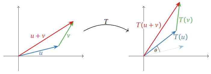
Figure \(\PageIndex{1}\)
For the second property, \(cT(u)\) is the vector obtained by rotating \(u\) by the angle \(\theta\text{,}\) then changing its length by a factor of \(c\) (reversing direction of \(c<0\). On the other hand, \(T(cu)\) first changes the length of \(c\text{,}\) then rotates. But it does not matter in which order we do these two operations.
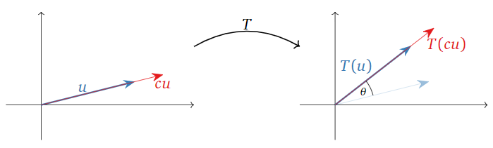
Figure \(\PageIndex{2}\)
This verifies that \(T\) is a linear transformation. We will find its matrix in the next Subsection The Matrix of a Linear Transformation. Note however that it is not at all obvious that \(T\) can be expressed as multiplication by a matrix.
Define \(T\colon\mathbb{R}^2\to\mathbb{R}^3 \) by the formula
\[T\left(\begin{array}{c}x\\y\end{array}\right)=\left(\begin{array}{c}3x-y\\y\\x\end{array}\right).\nonumber\]
Verify that \(T\) is linear.
Solution
We have to check the defining properties, Definition \(\PageIndex{1}\), for all vectors \(u,v\) and all scalars \(c\). In other words, we have to treat \(u,v,\) and \(c\) as unknowns; the only thing we are allowed to use is the definition of \(T\). Since \(T\) is defined in terms of the coordinates of \(u,v\text{,}\) we need to give those names as well; say \(u={x_1\choose y_1}\) and \(v={x_2\choose y_2}\). For the first property, we have
\[\begin{aligned} T\left(\left(\begin{array}{c}x_1\\y_1\end{array}\right)+\left(\begin{array}{c}x_2\\y_2\end{array}\right)\right)&=T\left(\begin{array}{c}x_1+x_2\\y_1+y_2\end{array}\right)=\left(\begin{array}{c}3(x_1+x_2)-(y_1+y_2) \\ y_1+y_2 \\ x_1+x_2\end{array}\right) \\ &=\left(\begin{array}{c} (3x_1-y_1)+(3x_2-y_2) \\ y_1+y_2 \\ x_1+x_2\end{array}\right) \\ &=\left(\begin{array}{c}3x_1-y_1 \\ y_1 \\ x_1\end{array}\right)+\left(\begin{array}{c}3x_2-y_2 \\ y_2\\x_2\end{array}\right)=T\left(\begin{array}{c}x_1\\y_1\end{array}\right)+T\left(\begin{array}{c}x_2\\y_2\end{array}\right).\end{aligned}\nonumber\]
For the second property,
\[\begin{aligned}T\left(c\left(\begin{array}{c}x_1\\y_1\end{array}\right)\right)&=T\left(\begin{array}{c}cx_1\\cy_1\end{array}\right)=\left(\begin{array}{c}3(cx_1)-(cy_1) \\ cy_1 \\ cx_1\end{array}\right) \\ &=\left(\begin{array}{c}c(3x_1-y_1)\\cy_1\\cx_1\end{array}\right)=c\left(\begin{array}{c}3x_1-y_1\\y_1\\x_1\end{array}\right)=cT\left(\begin{array}{c}x_1\\y_1\end{array}\right).\end{aligned}\]
Since \(T\) satisfies the defining properties, Definition \(\PageIndex{1}\), \(T\) is a linear transformation.
Note: we will see in this Example \(\PageIndex{9}\) below that
\[T\left(\begin{array}{c}x\\y\end{array}\right)=\left(\begin{array}{cc}3&-1\\0&1\\1&0\end{array}\right)\left(\begin{array}{c}x\\y\end{array}\right).\nonumber\]
Hence \(T\) is in fact a matrix transformation.
One can show that, if a transformation is defined by formulas in the coordinates as in the above example, then the transformation is linear if and only if each coordinate is a linear expression in the variables with no constant term.
Define \(T\colon\mathbb{R}^3 \to\mathbb{R}^3 \) by
\[ T(x) = x + \left(\begin{array}{c}1\\2\\3\end{array}\right). \nonumber \]
This kind of transformation is called a translation. As in a previous Example \(\PageIndex{1}\), this \(T\) is not linear, because \(T(0)\) is not the zero vector.
Verify that the following transformations from \(\mathbb{R}^2\) to \(\mathbb{R}^2\) are not linear:
\[T_1\left(\begin{array}{c}x\\y\end{array}\right)=\left(\begin{array}{c}|x|\\y\end{array}\right)\quad T_2\left(\begin{array}{c}x\\y\end{array}\right)=\left(\begin{array}{c}xy\\y\end{array}\right)\quad T_3\left(\begin{array}{c}x\\y\end{array}\right)=\left(\begin{array}{c}2x+1\\x-2y\end{array}\right).\nonumber\]
Solution
In order to verify that a transformation \(T\) is not linear, we have to show that \(T\) does not satisfy at least one of the two defining properties, Definition \(\PageIndex{1}\). For the first, the negation of the statement “\(T(u+v)=T(u)+T(v)\) for all vectors \(u,v\)” is “there exists at least one pair of vectors \(u,v\) such that \(T(u+v)\neq T(u)+T(v)\).” In other words, it suffices to find one example of a pair of vectors \(u,v\) such that \(T(u+v)\neq T(u)+T(v)\). Likewise, for the second, the negation of the statement “\(T(cu) = cT(u)\) for all vectors \(u\) and all scalars \(c\)” is “there exists some vector \(u\) and some scalar \(c\) such that \(T(cu)\neq cT(u)\).” In other words, it suffices to find one vector \(u\) and one scalar \(c\) such that \(T(cu)\neq cT(u)\).
For the first transformation, we note that
\[T_1\left(-\left(\begin{array}{c}1\\0\end{array}\right)\right)=T_1\left(\begin{array}{c}-1\\0\end{array}\right)=\left(\begin{array}{c}|-1|\\0\end{array}\right)=\left(\begin{array}{c}1\\0\end{array}\right)\nonumber\]
but that
\[-T_1\left(\begin{array}{c}1\\0\end{array}\right)=-\left(\begin{array}{c}|1|\\0\end{array}\right)=-\left(\begin{array}{c}1\\0\end{array}\right)=\left(\begin{array}{c}-1\\0\end{array}\right).\nonumber\]
Therefore, this transformation does not satisfy the second property.
For the second transformation, we note that
\[T_2\left(2\left(\begin{array}{c}1\\1\end{array}\right)\right)=T_2\left(\begin{array}{c}2\\2\end{array}\right)=\left(\begin{array}{c}2\cdot 2\\2\end{array}\right)=\left(\begin{array}{c}4\\2\end{array}\right)\nonumber\]
but that
\[2T_2\left(\begin{array}{c}1\\1\end{array}\right)=2\left(\begin{array}{c}1\cdot 1\\1\end{array}\right)=2\left(\begin{array}{c}1\\1\end{array}\right)=\left(\begin{array}{c}2\\2\end{array}\right).\nonumber\]
Therefore, this transformation does not satisfy the second property.
For the third transformation, we observe that
\[T_3\left(\begin{array}{c}0\\0\end{array}\right)=\left(\begin{array}{c}2(0)+1\\0-2(0)\end{array}\right)=\left(\begin{array}{c}1\\0\end{array}\right)\neq\left(\begin{array}{c}0\\0\end{array}\right).\nonumber\]
Since \(T_3\) does not take the zero vector to the zero vector, it cannot be linear.
When deciding whether a transformation \(T\) is linear, generally the first thing to do is to check whether \(T(0)=0\text{;}\) if not, \(T\) is automatically not linear. Note however that the non-linear transformations \(T_1\) and \(T_2\) of the above example do take the zero vector to the zero vector.
Find an example of a transformation that satisfies the first property of linearity, Definition \(\PageIndex{1}\), but not the second.
The Standard Coordinate Vectors
In the next subsection, we will present the relationship between linear transformations and matrix transformations. Before doing so, we need the following important notation.
The standard coordinate vectors in \(\mathbb{R}^n \) are the \(n\) vectors
\[e_1=\left(\begin{array}{c}1\\0\\ \vdots\\0\\0\end{array}\right),\quad e_2=\left(\begin{array}{c}0\\1\\ \vdots\\0\\0\end{array}\right),\quad\cdots ,\quad e_{n-1}=\left(\begin{array}{c}0\\0\\ \vdots\\1\\0\end{array}\right),\quad e_n=\left(\begin{array}{c}0\\0\\ \vdots\\0\\1\end{array}\right).\nonumber\]
The \(i\)th entry of \(e_i\) is equal to 1, and the other entries are zero.
From now on, for the rest of the book, we will use the symbols \(\color{red}e_1,e_2,\ldots\) to denote the standard coordinate vectors.
There is an ambiguity in this notation: one has to know from context that \(e_1\) is meant to have \(n\) entries. That is, the vectors
\[\left(\begin{array}{c}1\\0\end{array}\right)\quad\text{and}\quad\left(\begin{array}{c}1\\0\\0\end{array}\right)\nonumber\]
may both be denoted \(e_1\text{,}\) depending on whether we are discussing vectors in \(\mathbb{R}^2\) or in \(\mathbb{R}^3 \).
The standard coordinate vectors in \(\mathbb{R}^2\) and \(\mathbb{R}^3 \) are pictured below.
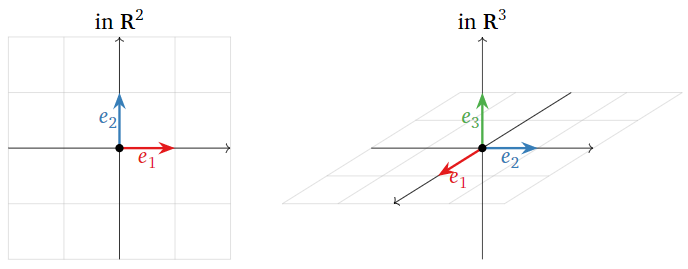
Figure \(\PageIndex{3}\)
These are the vectors of length 1 that point in the positive directions of each of the axes.
If \(A\) is an \(m\times n\) matrix with columns \(v_1,v_2,\ldots,v_m\text{,}\) then \(\color{red}Ae_i = v_i\) for each \(i=1,2,\ldots,n\text{:}\)
\[\left(\begin{array}{cccc}|&|&\quad &| \\ v_1&v_2&\quad &v_n \\ |&|&\quad &|\end{array}\right)e_i=v_i.\nonumber\]
In other words, multiplying a matrix by \(e_i\) simply selects its \(i\)th column.
For example,
\[\left(\begin{array}{ccc}1&2&3\\4&5&6\\7&8&9\end{array}\right)\:\left(\begin{array}{c}1\\0\\0\end{array}\right)=\left(\begin{array}{c}1\\4\\7\end{array}\right)\quad\left(\begin{array}{ccc}1&2&3\\4&5&6\\7&8&9\end{array}\right)\:\left(\begin{array}{c}0\\1\\0\end{array}\right)=\left(\begin{array}{c}2\\5\\8\end{array}\right)\quad\left(\begin{array}{ccc}1&2&3\\4&5&6\\7&8&9\end{array}\right)\:\left(\begin{array}{c}0\\0\\01\end{array}\right)=\left(\begin{array}{c}3\\6\\9\end{array}\right).\nonumber\]
The \(n\times n\) identity matrix is the matrix \(I_n\) whose columns are the \(n\) standard coordinate vectors in \(\mathbb{R}^n \text{:}\)
\[I_n=\left(\begin{array}{ccccc}1&0&\cdots &0&0 \\ 0&1&\cdots &0&0 \\ \vdots &\vdots &\ddots &\vdots &\vdots \\ 0&0&\cdots &1&0 \\ 0&0&\cdots &0&1\end{array}\right).\nonumber\]
We will see in this Example \(\PageIndex{10}\) below that the identity matrix is the matrix of the identity transformation, Definition 3.1.2.
The Matrix of a Linear Transformation
Now we can prove that every linear transformation is a matrix transformation, and we will show how to compute the matrix.
Let \(T\colon\mathbb{R}^n \to\mathbb{R}^m \) be a linear transformation. Let \(A\) be the \(m\times n\) matrix
\[A=\left(\begin{array}{cccc}|&|&\quad&| \\ T(e_1)&T(e_2)&\cdots&T(e_n) \\ |&|&\quad&|\end{array}\right).\nonumber\]
Then \(T\) is the matrix transformation associated with \(A\text{:}\) that is, \(T(x) = Ax\).
- Proof
-
We suppose for simplicity that \(T\) is a transformation from \(\mathbb{R}^3 \) to \(\mathbb{R}^2\). Let \(A\) be the matrix given in the statement of the theorem. Then
\[\begin{aligned}T\left(\begin{array}{c}x\\y\\z\end{array}\right);&=T\left(x\left(\begin{array}{c}1\\0\\0\end{array}\right)+y\left(\begin{array}{c}0\\1\\0\end{array}\right)+z\left(\begin{array}{c}0\\0\\1\end{array}\right)\right) \\ &=T(xe_1+ye_2+ze_3) \\ &=xT(e_1)+yT(e_2)+zT(e_3) \\ &=\left(\begin{array}{ccc}|&|&| \\ T(e_1)&T(e_2)&T(e_3) \\ |&|&|\end{array}\right)\:\left(\begin{array}{c}x\\y\\z\end{array}\right) \\ &=A\left(\begin{array}{c}x\\y\\z\end{array}\right).\end{aligned}\nonumber\]
The matrix \(A\) in the above theorem is called the standard matrix for \(T\). The columns of \(A\) are the vectors obtained by evaluating \(T\) on the \(n\) standard coordinate vectors in \(\mathbb{R}^n \). To summarize part of the theorem:
Matrix transformations are the same as linear transformations.
Linear transformations are the same as matrix transformations, which come from matrices. The correspondence can be summarized in the following dictionary.
\[\begin{aligned} \begin{array}{c}T:\mathbb{R}^n\to\mathbb{R}^m \\ {\text{Linear transformation}}\end{array}\quad &\longrightarrow m\times n\text{ matrix }A=\left(\begin{array}{cccc}|&|&\quad&| \\ T(e_1)&T(e_2)&\cdots &T(e_n) \\ |&|&\quad&|\end{array}\right) \\ \begin{array}{c}T:\mathbb{R}^n\to\mathbb{R}^m \\ T(x)=Ax\end{array} \quad &\longleftarrow m\times n\text{ matrix }A\end{aligned}\]
Define \(T\colon\mathbb{R}^2\to\mathbb{R}^2\) by \(T(x)=1.5x\). Find the standard matrix \(A\) for \(T\).
Solution
The columns of \(A\) are obtained by evaluating \(T\) on the standard coordinate vectors \(e_1,e_2\).
\[ \left.\begin{aligned} T(e_1) \amp= 1.5e_1 = \left(\begin{array}{c}1.5\\0\end{array}\right) \\ T(e_2) \amp= 1.5e_2 = \left(\begin{array}{c}0\\1.5\end{array}\right) \end{aligned}\right\} \implies A = \left(\begin{array}{cc}1.5&0\\0&1.5\end{array}\right). \nonumber \]
This is the matrix we started with in Example 3.1.5 in Section 3.1.
Define \(T\colon\mathbb{R}^2\to\mathbb{R}^2\) by
\[ T(x) = \text{ the vector $x$ rotated counterclockwise by the angle $\theta$}. \nonumber \]
Find the standard matrix for \(T\).
Solution
The columns of \(A\) are obtained by evaluating \(T\) on the standard coordinate vectors \(e_1,e_2\). In order to compute the entries of \(T(e_1)\) and \(T(e_2)\text{,}\) we have to do some trigonometry.
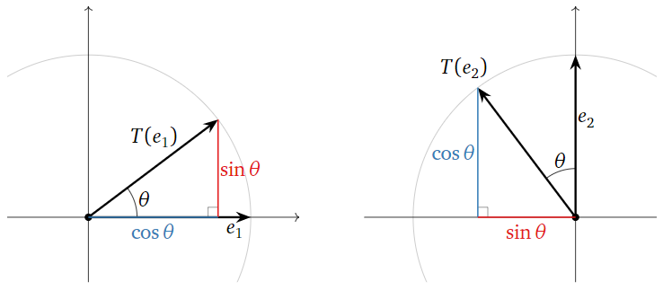
Figure \(\PageIndex{4}\)
We see from the picture that
\[\left.\begin{aligned} T(e_1)&=\left(\begin{array}{c}\color{blue}{\cos\theta}\\ \color{red}{\sin\theta}\end{array}\right) \\ T(e_2)&=\left(\begin{array}{c}{\color{black}{-}\color{red}{\sin\theta}}\\ \color{blue}{\cos\theta}\end{array}\right)\end{aligned}\right\} \implies A=\left(\begin{array}{cc}\color{blue}{\cos\theta}&\color{black}{-}\color{red}{\sin\theta} \\ \color{red}{\sin\theta}&\color{blue}{\cos\theta}\end{array}\right)\nonumber\]
We saw in the above example that the matrix for counterclockwise rotation of the plane by an angle of \(\theta\) is
\[A=\left(\begin{array}{cc}\cos\theta &-\sin\theta \\ \sin\theta &\cos\theta\end{array}\right).\nonumber\]
Define \(T\colon\mathbb{R}^2\to\mathbb{R}^3 \) by the formula
\[T\left(\begin{array}{c}x\\y\end{array}\right)=\left(\begin{array}{c}3x-y\\y\\x\end{array}\right).\nonumber\]
Find the standard matrix for \(T\).
Solution
We substitute the standard coordinate vectors into the formula defining \(T\text{:}\)
\[\left.\begin{aligned} T(e_1)&=T\left(\begin{array}{c}1\\0\end{array}\right)=\left(\begin{array}{c}3(1)-0\\0\\1\end{array}\right)=\left(\begin{array}{c}3\\0\\1\end{array}\right) \\ T(e_2)&=T\left(\begin{array}{c}0\\1\end{array}\right)=\left(\begin{array}{c}3(0)-1\\1\\0\end{array}\right)=\left(\begin{array}{c}-1\\1\\0\end{array}\right)\end{aligned}\right\}\implies A=\left(\begin{array}{cc}3&-1\\0&1\\1&0\end{array}\right).\nonumber\]
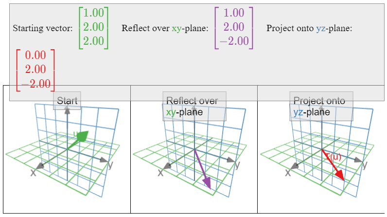
Let \(T\colon\mathbb{R}^3 \to\mathbb{R}^3 \) be the linear transformation that reflects over the \(xy\)-plane and then projects onto the \(yz\)-plane. What is the standard matrix for \(T\text{?}\)
Solution
This transformation is described geometrically, in two steps. To find the columns of \(A\text{,}\) we need to follow the standard coordinate vectors through each of these steps.
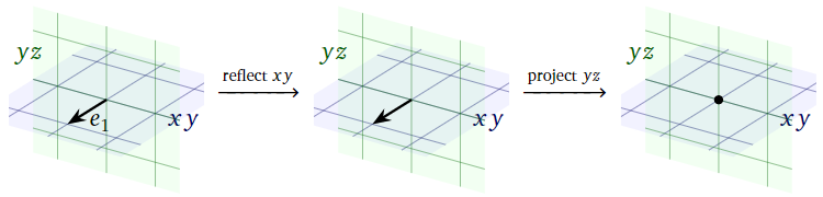
Figure \(\PageIndex{5}\)
Since \(e_1\) lies on the \(xy\)-plane, reflecting over the \(xy\)-plane does not move \(e_1\). Since \(e_1\) is perpendicular to the \(yz\)-plane, projecting \(e_1\) onto the \(yz\)-plane sends it to zero. Therefore,
\[ T(e_1) = \left(\begin{array}{c}0\\0\\0\end{array}\right). \nonumber \]
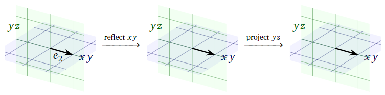
Figure \(\PageIndex{6}\)
Since \(e_2\) lies on the \(xy\)-plane, reflecting over the \(xy\)-plane does not move \(e_2\). Since \(e_2\) lies on the \(yz\)-plane, projecting onto the \(yz\)-plane does not move \(e_2\) either. Therefore,
\[ T(e_2) = e_2 = \left(\begin{array}{c}0\\1\\0\end{array}\right). \nonumber \]
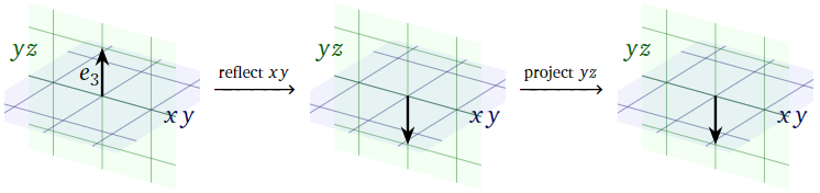
Figure \(\PageIndex{7}\)
Since \(e_3\) is perpendicular to the \(xy\)-plane, reflecting over the \(xy\)-plane takes \(e_3\) to its negative. Since \(-e_3\) lies on the \(yz\)-plane, projecting onto the \(yz\)-plane does not move it. Therefore,
\[ T(e_3) = -e_3 = \left(\begin{array}{c}0\\0\\-1\end{array}\right). \nonumber \]
Now we have computed all three columns of \(A\text{:}\)
\[\left.\begin{aligned} T(e_1)&=\left(\begin{array}{c}0\\0\\0\end{array}\right) \\ T(e_2)&=\left(\begin{array}{c}0\\1\\0\end{array}\right) \\ T(e_1)&=\left(\begin{array}{c}0\\0\\-1\end{array}\right) \end{aligned}\right\} \implies A=\left(\begin{array}{ccc}0&0&0\\0&1&0\\0&0&-1\end{array}\right).\nonumber\]
Recall from Definition 3.1.2 in Section 3.1 that the identity transformation is the transformation \(\text{Id}_{\mathbb{R}^n }\colon\mathbb{R}^n \to\mathbb{R}^n \) defined by \(\text{Id}_{\mathbb{R}^n }(x) = x\) for every vector \(x\).
Verify that the identity transformation \(\text{Id}_{\mathbb{R}^n }\colon\mathbb{R}^n \to\mathbb{R}^n \) is linear, and compute its standard matrix.
Solution
We verify the two defining properties, Definition \(\PageIndex{1}\), of linear transformations. Let \(u,v\) be vectors in \(\mathbb{R}^n \). Then
\[\text{Id}_{\mathbb{R}^n}(u+v)=u+v=\text{Id}_{\mathbb{R}^n}(u)+\text{Id}_{\mathbb{R}^n}(v).\nonumber\]
If \(c\) is a scalar, then
\[ \text{Id}_{\mathbb{R}^n }(cu) = cu = c\text{Id}_{\mathbb{R}^n }(u). \nonumber \]
Since \(\text{Id}_{\mathbb{R}^n }\) satisfies the two defining properties, it is a linear transformation.
Now that we know that \(\text{Id}_{\mathbb{R}^n }\) is linear, it makes sense to compute its standard matrix. For each standard coordinate vector \(e_i\text{,}\) we have \(\text{Id}_{R^n}(e_i) = e_i\). In other words, the columns of the standard matrix of \(\text{Id}_{\mathbb{R}^n }\) are the standard coordinate vectors, so the standard matrix is the identity matrix
\[I_n=\left(\begin{array}{ccccc}1&0&\cdots&0&0\\0&1&\cdots&0&0\\ \vdots&\vdots&\ddots&\vdots&\vdots \\ 0&0&\cdots &1&1\\0&0&\cdots &0&1\end{array}\right).\nonumber\]
We computed in Example \(\PageIndex{11}\) that the matrix of the identity transform is the identity matrix: for every \(x\) in \(\mathbb{R}^n \text{,}\)
\[ x = \text{Id}_{\mathbb{R}^n }(x) = I_nx. \nonumber \]
Therefore, \(I_nx=x\) for all vectors \(x\text{:}\) the product of the identity matrix and a vector is the same vector.