3.0: Prelude to Linear Transformations and Matrix Algebra

Last updated
Save as PDF

Page ID: 78171

$ \newcommand{\vecs}[1]{\overset { \scriptstyle \rightharpoonup} {\mathbf{#1}} } $ $ \newcommand{\vecd}[1]{\overset{-\!-\!\rightharpoonup}{\vphantom{a}\smash {#1}}} $$\newcommand{\id}{\mathrm{id}}$ $ \newcommand{\Span}{\mathrm{span}}$ $ \newcommand{\kernel}{\mathrm{null}\,}$ $ \newcommand{\range}{\mathrm{range}\,}$ $ \newcommand{\RealPart}{\mathrm{Re}}$ $ \newcommand{\ImaginaryPart}{\mathrm{Im}}$ $ \newcommand{\Argument}{\mathrm{Arg}}$ $ \newcommand{\norm}[1]{\| #1 \|}$ $ \newcommand{\inner}[2]{\langle #1, #2 \rangle}$ $ \newcommand{\Span}{\mathrm{span}}$ $\newcommand{\id}{\mathrm{id}}$ $ \newcommand{\Span}{\mathrm{span}}$ $ \newcommand{\kernel}{\mathrm{null}\,}$ $ \newcommand{\range}{\mathrm{range}\,}$ $ \newcommand{\RealPart}{\mathrm{Re}}$ $ \newcommand{\ImaginaryPart}{\mathrm{Im}}$ $ \newcommand{\Argument}{\mathrm{Arg}}$ $ \newcommand{\norm}[1]{\| #1 \|}$ $ \newcommand{\inner}[2]{\langle #1, #2 \rangle}$ $ \newcommand{\Span}{\mathrm{span}}$$\newcommand{\AA}{\unicode[.8,0]{x212B}}$

Example $\PageIndex{1}$

Suppose you are building a robot arm with three joints that can move its hand around a plane, as in the following picture.

$162682942668943594.png$

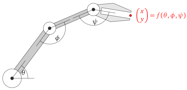
Figure $\PageIndex{1}$

Jun 23, 2021, 12:13 PM

\usetikzlibrary{ipe} \usetikzlibrary{angles} \tikzstyle{ipe stylesheet} = [ ipe import, even odd rule, line join=round, line cap=butt, ipe pen normal/.style={line width=0.4}, ipe pen heavier/.style={line width=0.8}, ipe pen fat/.style={line width=1.2}, ipe pen ultrafat/.style={line width=2}, ipe pen normal, ipe mark normal/.style={ipe mark scale=3}, ipe mark large/.style={ipe mark scale=5}, ipe mark small/.style={ipe mark scale=2}, ipe mark tiny/.style={ipe mark scale=1.1}, ipe mark normal, /pgf/arrow keys/.cd, ipe arrow normal/.style={scale=7}, ipe arrow large/.style={scale=10}, ipe arrow small/.style={scale=5}, ipe arrow tiny/.style={scale=3}, ipe arrow normal, /tikz/.cd, ipe arrows, % update arrows <->/.tip = ipe normal, ipe dash normal/.style={dash pattern=}, ipe dash dashed/.style={dash pattern=on 4bp off 4bp}, ipe dash dotted/.style={dash pattern=on 1bp off 3bp}, ipe dash dash dotted/.style={dash pattern=on 4bp off 2bp on 1bp off 2bp}, ipe dash dash dot dotted/.style={dash pattern=on 4bp off 2bp on 1bp off 2bp on 1bp off 2bp}, ipe dash normal, ipe node/.append style={font=\normalsize}, ipe stretch normal/.style={ipe node stretch=1}, ipe stretch normal, ipe opacity 10/.style={opacity=0.1}, ipe opacity 30/.style={opacity=0.3}, ipe opacity 50/.style={opacity=0.5}, ipe opacity 75/.style={opacity=0.75}, ipe opacity opaque/.style={opacity=1}, ipe opacity opaque, ] \begin{tikzpicture}[ipe stylesheet, scale=.7] \draw[fill=white!80!black] (100, 528) -- (196, 656) -- (220, 656) -- (124, 528) -- cycle; \draw[fill=white!80!black] (208, 664) -- (320, 712) -- (320, 696) -- (208, 648) -- cycle; \begin{scope}[shift={(321.91, 715.847)}, rotate=-9.1623] \draw[fill=white!90!black] (0, 0) -- (48, 12) -- (96, 0) -- (96, -4) -- (20, -4) -- (20, -20) -- (96, -20) -- (96, -24) -- (48, -36) -- (0, -24) -- cycle; \draw[fill=red] (96, -12) circle[radius=1mm] node[right=2mm, red] {$\vec{x y} = f(\theta,\phi,\psi)$}; \end{scope} \filldraw[fill=white] (208, 656) circle[radius=16]; \filldraw[fill=white] (320, 704) circle[radius=16]; \filldraw[fill=white] (112, 528) circle[radius=24]; \filldraw[white!20!black] (112, 528) circle[radius=4] (208, 656) circle[radius=4] (320, 704) circle[radius=4]; \coordinate (c1) at (112, 528); \coordinate (c2) at (208, 656); \coordinate (c3) at (320, 704); \coordinate (x1) at ($(c1) + (2cm,0)$); \coordinate (x3) at ($(c3) + (2cm,0)$); \draw (c1) -- (x1); \draw (c1) -- ($(c1)!2cm!(c2)$); \pic[draw, "$\theta$", angle radius=1cm, angle eccentricity=.8] {angle=x1--c1--c2}; \draw (c2) -- ($(c2)!2cm!(c1)$); \draw (c2) -- ($(c2)!2cm!(c3)$); \pic[draw, "$\phi$", angle radius=1cm, angle eccentricity=.8] {angle=c1--c2--c3}; \coordinate (x3p) at ($(c3)!2cm!-9.1623:(x3)$); \draw (c3) -- ($(c3)!2cm!(c2)$); \draw (c3) -- (x3p); \pic[draw, "$\psi$", angle radius=1cm, angle eccentricity=.8] {angle=c2--c3--x3p}; \end{tikzpicture}

Define a transformation $f$ as follows: $f(\theta,\phi,\psi)$ is the $(x,y)$ position of the hand when the joints are rotated by angles $\theta, \phi, \psi\text{,}$ respectively. The output of $f$ tells you where the hand will be on the plane when the joints are set at the given input angles.

Unfortunately, this kind of function does not come from a matrix, so one cannot use linear algebra to answer questions about this function. In fact, these functions are rather complicated; their study is the subject of inverse kinematics.

In this chapter, we will be concerned with the relationship between matrices and transformations. In Section 3.1, we will consider the equation $b = Ax$ as a function with independent variable $x$ and dependent variable $b\text{,}$ and we draw pictures accordingly. We spend some time studying transformations in the abstract, and asking questions about a transformation, like whether it is one-to-one and/or onto (Section 3.2). In Section 3.3 we will answer the question: “when exactly can a transformation be expressed by a matrix?” We then present matrix multiplication as a special case of composition of transformations (Section 3.4). This leads to the study of matrix algebra: that is, to what extent one can do arithmetic with matrices in the place of numbers. With this in place, we learn to solve matrix equations by dividing by a matrix in Section 3.5.