
3.5: Matrix Inverses
- Page ID
- 70199

- Understand what it means for a square matrix to be invertible.
- Learn about invertible transformations, and understand the relationship between invertible matrices and invertible transformations.
- Recipes: compute the inverse matrix, solve a linear system by taking inverses.
- Picture: the inverse of a transformation.
- Vocabulary words: inverse matrix, inverse transformation.
In Section 3.1 we learned to multiply matrices together. In this section, we learn to “divide” by a matrix. This allows us to solve the matrix equation \(Ax=b\) in an elegant way:
\[ Ax = b \quad\iff\quad x = A^{-1} b. \nonumber \]
One has to take care when “dividing by matrices”, however, because not every matrix has an inverse, and the order of matrix multiplication is important.
Invertible Matrices
The reciprocal or inverse of a nonzero number \(a\) is the number \(b\) which is characterized by the property that \(ab = 1\). For instance, the inverse of \(7\) is \(1/7\). We use this formulation to define the inverse of a matrix.
Let \(A\) be an \(n\times n\) (square) matrix. We say that \(A\) is invertible if there is an \(n\times n\) matrix \(B\) such that
\[ AB = I_n \quad\text{and}\quad BA = I_n. \nonumber \]
In this case, the matrix \(B\) is called the inverse of \(A\text{,}\) and we write \(B = A^{-1}\).
We have to require \(AB = I_n\) and \(BA = I_n\) because in general matrix multiplication is not commutative. However, we will show in Corollary 3.6.1 in Section 3.6 that if \(A\) and \(B\) are \(n\times n\) matrices such that \(AB = I_n\text{,}\) then automatically \(BA = I_n\).
Verify that the matrices
\[A=\left(\begin{array}{cc}2&1\\1&1\end{array}\right)\quad\text{and}\quad B=\left(\begin{array}{cc}1&-1\\-1&2\end{array}\right)\nonumber\]
are inverses.
Solution
We will check that \(AB = I_2\) and that \(BA = I_2\).
\[\begin{aligned}AB&=\left(\begin{array}{cc}2&1\\1&1\end{array}\right)\left(\begin{array}{cc}1&-1\\-1&2\end{array}\right)=\left(\begin{array}{cc}1&0\\0&1\end{array}\right) \\ BA&=\left(\begin{array}{cc}1&-1\\-1&2\end{array}\right)\left(\begin{array}{cc}2&1\\1&1\end{array}\right)=\left(\begin{array}{cc}1&0\\0&1\end{array}\right)\end{aligned}\]
Therefore, \(A\) is invertible, with inverse \(B\).
There exist non-square matrices whose product is the identity. Indeed, if
\[A=\left(\begin{array}{ccc}1&0&0\\0&1&0\end{array}\right)\quad\text{and}\quad B=\left(\begin{array}{cc}1&0\\0&1\\0&0\end{array}\right)\nonumber\]
then \(AB = I_2.\) However, \(BA\neq I_3\text{,}\) so \(B\) does not deserve to be called the inverse of \(A\).
One can show using the ideas later in this section that if \(A\) is an \(n\times m\) matrix for \(n\neq m\text{,}\) then there is no \(m\times n\) matrix \(B\) such that \(AB = I_m\) and \(BA = I_n\). For this reason, we restrict ourselves to square matrices when we discuss matrix invertibility.
Let \(A\) and \(B\) be invertible \(n\times n\) matrices.
- \(A^{-1}\) is invertible, and its inverse is \((A^{-1}){}^{-1} = A.\)
- \(AB\) is invertible, and its inverse is \((AB)^{-1} = B^{-1} A^{-1}\) (note the order).
- Proof
-
- The equations \(AA^{-1}=I_n\) and \(A^{-1}A = I_n\) at the same time exhibit \(A^{-1}\) as the inverse of \(A\) and \(A\) as the inverse of \(A^{-1}.\)
- We compute
\[ (B^{-1} A^{-1})AB = B^{-1}(A^{-1} A)B = B^{-1} I_n B = B^{-1} B = I_n. \nonumber \]
Here we used the associativity of matrix multiplication and the fact that \(I_n B = B\). This shows that \(B^{-1} A^{-1}\) is the inverse of \(AB\).
Why is the inverse of \(AB\) not equal to \(A^{-1} B^{-1}\text{?}\) If it were, then we would have
\[ I_n = (AB)(A^{-1} B^{-1}) = ABA^{-1} B^{-1}. \nonumber \]
But there is no reason for \(ABA^{-1} B^{-1}\) to equal the identity matrix: one cannot switch the order of \(A^{-1}\) and \(B\text{,}\) so there is nothing to cancel in this expression. In fact, if \(I_n = (AB)(A^{-1} B^{-1})\text{,}\) then we can multiply both sides on the right by \(BA\) to conclude that \(AB = BA\). In other words, \((AB)^{-1} = A^{-1} B^{-1}\) if and only if \(AB=BA\).
More generally, the inverse of a product of several invertible matrices is the product of the inverses, in the opposite order; the proof is the same. For instance,
\[ (ABC)^{-1} = C^{-1} B^{-1} A^{-1}. \nonumber \]
Computing the Inverse Matrix
So far we have defined the inverse matrix without giving any strategy for computing it. We do so now, beginning with the special case of \(2\times 2\) matrices. Then we will give a recipe for the \(n\times n\) case.
The determinant of a \(2\times 2\) matrix is the number
\[\text{det}\left(\begin{array}{cc}a&b\\c&d\end{array}\right)=ad-bc.\nonumber\]
Let \(A=\left(\begin{array}{cc}a&b\\c&d\end{array}\right)\).
- If \(\det(A) \neq 0\text{,}\) then \(A\) is invertible, and
\[ A^{-1} = \frac 1{\det(A)}\left(\begin{array}{cc}d&-b\\-c&a\end{array}\right). \nonumber \] - If \(\det(A) = 0,\) then \(A\) is not invertible.
- Proof
-
- Suppose that \(\det(A)\neq 0\). Define \(\displaystyle B = \frac 1{\det(A)}\left(\begin{array}{cc}d&-b\\-c&a\end{array}\right).\) Then
\[ AB = \left(\begin{array}{cc}a&b\\c&d\end{array}\right) \frac 1{\det(A)}\left(\begin{array}{cc}d&-b\\-c&a\end{array}\right) = \frac 1{ad-bc}\left(\begin{array}{cc}ad-bc&0\\0&ad-bc\end{array}\right) = I_2. \nonumber \]
The reader can check that \(BA = I_2\text{,}\) so \(A\) is invertible and \(B = A^{-1}\). - Suppose that \(\det(A) = ad-bc = 0\). Let \(T\colon\mathbb{R}^2 \to\mathbb{R}^2 \) be the matrix transformation \(T(x) = Ax\). Then
\[\begin{aligned}T\left(\begin{array}{c}-b\\a\end{array}\right)&=\left(\begin{array}{cc}a&b\\c&d\end{array}\right)\left(\begin{array}{c}-b\\a\end{array}\right)=\left(\begin{array}{cc}-ab+ab\\-bc+ad\end{array}\right)=\left(\begin{array}{c}0\\ \det(A)\end{array}\right)=0 \\ T\left(\begin{array}{c}d\\-c\end{array}\right)&=\left(\begin{array}{cc}a&b\\c&d\end{array}\right)\left(\begin{array}{c}d\\-c\end{array}\right)=\left(\begin{array}{c}ad-bc\\cd-cd\end{array}\right)=\left(\begin{array}{c}\det(A)\\0\end{array}\right)=0.\end{aligned}\]
If \(A\) is the zero matrix, then it is obviously not invertible. Otherwise, one of \(v= {-b\choose a}\) and \(v = {d\choose -c}\) will be a nonzero vector in the null space of \(A\). Suppose that there were a matrix \(B\) such that \(BA=I_2\). Then
\[ v = I_2v = BAv = B0 = 0, \nonumber \]
which is impossible as \(v\neq 0\). Therefore, \(A\) is not invertible.
- Suppose that \(\det(A)\neq 0\). Define \(\displaystyle B = \frac 1{\det(A)}\left(\begin{array}{cc}d&-b\\-c&a\end{array}\right).\) Then
There is an analogous formula for the inverse of an \(n\times n\) matrix, but it is not as simple, and it is computationally intensive. The interested reader can find it in Subsection Cramer's Rule and Matrix Inverses in Section 4.2.
Let
\[ A = \left(\begin{array}{cc}1&2\\3&4\end{array}\right). \nonumber \]
Then \(\det(A) = 1\cdot 4 - 2\cdot 3 = -2.\) By the Proposition \(\PageIndex{1}\), the matrix \(A\) is invertible with inverse
\[\left(\begin{array}{cc}1&2\\3&4\end{array}\right)^{-1}=\frac{1}{\det(A)}\left(\begin{array}{cc}4&-2\\-3&1\end{array}\right)=-\frac{1}{2}\left(\begin{array}{cc}4&-2\\-3&1\end{array}\right).\nonumber\]
We check:
\[\left(\begin{array}{cc}1&2\\3&4\end{array}\right)\cdot -\frac{1}{2}\left(\begin{array}{cc}4&-2\\-3&1\end{array}\right)=-\frac{1}{2}\left(\begin{array}{cc}-2&0\\0&-2\end{array}\right)=I_2.\nonumber\]
The following theorem gives a procedure for computing \(A^{-1}\) in general.
Let \(A\) be an \(n\times n\) matrix, and let \((\,A\mid I_n\,)\) be the matrix obtained by augmenting \(A\) by the identity matrix. If the reduced row echelon form of \((\,A\mid I_n\,)\) has the form \((\,I_n\mid B\,)\text{,}\) then \(A\) is invertible and \(B = A^{-1}\). Otherwise, \(A\) is not invertible.
- Proof
-
First suppose that the reduced row echelon form of \((\,A\mid I_n\,)\) does not have the form \((\,I_n\mid B\,)\). This means that fewer than \(n\) pivots are contained in the first \(n\) columns (the non-augmented part), so \(A\) has fewer than \(n\) pivots. It follows that \(\text{Nul}(A)\neq\{0\}\) (the equation \(Ax=0\) has a free variable), so there exists a nonzero vector \(v\) in \(\text{Nul}(A)\). Suppose that there were a matrix \(B\) such that \(BA=I_n\). Then
\[ v = I_nv = BAv = B0 = 0, \nonumber \]
which is impossible as \(v\neq 0\). Therefore, \(A\) is not invertible.
Now suppose that the reduced row echelon form of \((\,A\mid I_n\,)\) has the form \((\,I_n\mid B\,)\). In this case, all pivots are contained in the non-augmented part of the matrix, so the augmented part plays no role in the row reduction: the entries of the augmented part do not influence the choice of row operations used. Hence, row reducing \((\,A\mid I_n\,)\) is equivalent to solving the \(n\) systems of linear equations \(Ax_1 = e_1,\,Ax_2=e_2,\,\ldots,Ax_n=e_n\text{,}\) where \(e_1,e_2,\ldots,e_n\) are the standard coordinate vectors, Note 3.3.2 in Section 3.3:
\[\begin{aligned} Ax_1=\color{blue}{e_1}\color{black}{:}\quad &\left(\begin{array}{ccc|ccc}1&0&4&\color{blue}{1}&\color{gray}{0}&\color{gray}{0} \\ 0&1&2&\color{blue}{0}&\color{gray}{1}&\color{gray}{0} \\ 0&-3&-4&\color{blue}{0}&\color{gray}{0}&\color{gray}{1}\end{array}\right) \\ Ax_2=\color{red}{e_2}\color{black}{:}\quad &\left(\begin{array}{ccc|ccc}1&0&4&\color{gray}{1}&\color{red}{0}&\color{gray}{0}\\0&1&2&\color{gray}{0}&\color{red}{1}&\color{gray}{0} \\ 0&-3&-4&\color{gray}{0}&\color{red}{0}&\color{gray}{1}\end{array}\right) \\ Ax_3=\color{Green}{e_3}\color{black}{:}\quad &\left(\begin{array}{ccc|ccc}1&0&4&\color{gray}{1}&\color{gray}{0}&\color{Green}{0}\\0&1&2&\color{gray}{0}&\color{gray}{1}&\color{Green}{0}\\0&-3&-4&\color{gray}{0}&\color{gray}{0}&\color{Green}{1}\end{array}\right).\end{aligned}\]
The columns \(x_1,x_2,\ldots,x_n\) of the matrix \(B\) in the row reduced form are the solutions to these equations:
\[\begin{aligned} A\color{blue}{\left(\begin{array}{c}1\\0\\0\end{array}\right)}\color{black}{=e_1:}\quad &\left(\begin{array}{ccc|ccc}1&0&0&\color{blue}{1}&\color{gray}{-6}&\color{gray}{-2} \\ 0&1&0&\color{blue}{0}&\color{gray}{-2}&\color{gray}{-1}\\ 0&0&1&\color{blue}{0}&\color{gray}{3/2}&\color{gray}{1/2}\end{array}\right) \\ A\color{red}{\left(\begin{array}{c}-6\\-2\\3/2\end{array}\right)}\color{black}{=e_2:}\quad &\left(\begin{array}{ccc|ccc}1&0&0&\color{gray}{1}&\color{red}{-6}&\color{gray}{-2}\\0&1&0&\color{gray}{0}&\color{red}{-2}&\color{gray}{-1}\\ 0&0&1&\color{gray}{0}&\color{red}{3/2}&\color{gray}{1/2}\end{array}\right) \\ A\color{Green}{\left(\begin{array}{c}-2\\-1\\1/2\end{array}\right)}\color{black}{=e_3:}\quad &\left(\begin{array}{ccc|ccc}1&0&0&\color{gray}{1}&\color{gray}{-6}&\color{Green}{-2}\\ 0&1&0&\color{gray}{0}&\color{gray}{-2}&\color{Green}{-1}\\ 0&0&1&\color{gray}{0}&\color{gray}{3/2}&\color{Green}{1/2}\end{array}\right).\end{aligned}\]
By Fact 3.3.2 in Section 3.3, the product \(Be_i\) is just the \(i\)th column \(x_i\) of \(B\text{,}\) so
\[ e_i = Ax_i = ABe_i \nonumber \]
for all \(i\). By the same fact, the \(i\)th column of \(AB\) is \(e_i\text{,}\) which means that \(AB\) is the identity matrix. Thus \(B\) is the inverse of \(A\).
Find the inverse of the matrix
\[ A = \left(\begin{array}{ccc}1&0&4\\0&1&2\\0&-3&-4\end{array}\right). \nonumber \]
Solution
We augment by the identity and row reduce:
\[\begin{aligned}\left(\begin{array}{ccc|ccc}1&0&4&1&0&0\\0&1&2&0&1&0\\0&-3&-4&0&0&1\end{array}\right) \quad\xrightarrow{R_3=R_3+3R_2}\quad &\left(\begin{array}{ccc|ccc}1&0&4&1&0&0\\0&1&2&0&1&0\\0&\color{red}{0}&\color{red}{2}&\color{black}{0}&\color{red}{3}&\color{black}{1}\end{array}\right) \\ {}\xrightarrow{\begin{array}{l}{R_1=R_1-2R_3}\\{R_2=R_2-R_3}\end{array}}\quad &\left(\begin{array}{ccc|ccc}1&0&\color{red}{0}&\color{black}{1}&\color{red}{-6}&\color{red}{-2} \\ 0&1&\color{red}{0}&\color{black}{0}&\color{red}{-2}&\color{red}{-1} \\ 0&0&2&0&3&1\end{array}\right) \\ {}\xrightarrow{R_3=R_3\div 2}\quad &\left(\begin{array}{ccc|ccc}1&0&0&1&-6&-2 \\ 0&1&0&0&-2&-1 \\ 0&0&\color{red}{1}&\color{black}{0}&\color{red}{3/2}&\color{red}{1/2}\end{array}\right).\end{aligned}\]
By the Theorem \(\PageIndex{1}\), the inverse matrix is
\[\left(\begin{array}{ccc}1&0&4\\0&1&2\\0&-3&-4\end{array}\right)^{-1}=\left(\begin{array}{ccc}1&-6&-2\\0&-2&-1\\0&3/2&1/2\end{array}\right).\nonumber\]
We check:
\[\left(\begin{array}{ccc}1&0&4\\0&1&2\\0&-3&-4\end{array}\right)\left(\begin{array}{ccc}1&-6&-2\\0&-2&-1\\0&3/2&1/2\end{array}\right)=\left(\begin{array}{ccc}1&0&0\\0&1&0\\0&0&1\end{array}\right).\nonumber\]
Is the following matrix invertible?
\[A=\left(\begin{array}{ccc}1&0&4\\0&1&2\\0&-3&-6\end{array}\right).\nonumber\]
Solution
We augment by the identity and row reduce:
\[\left(\begin{array}{ccc|ccc}1&0&4&1&0&0\\0&1&2&0&1&0\\0&-3&-6&0&0&1\end{array}\right)\quad\xrightarrow{R_3=R_3+3R_2}\quad\left(\begin{array}{ccc|ccc}1&0&4&1&0&0\\0&1&2&0&1&0\\0&\color{red}{0}&\color{red}{0}&\color{black}{0}&\color{black}{3}&\color{black}{1}\end{array}\right).\nonumber\]
At this point we can stop, because it is clear that the reduced row echelon form will not have \(I_3\) in the non-augmented part: it will have a row of zeros. By the Theorem \(\PageIndex{1}\), the matrix is not invertible.
Solving Linear Systems using Inverses
In this subsection, we learn to solve \(Ax=b\) by “dividing by \(A\).”
Let \(A\) be an invertible \(n\times n\) matrix, and let \(b\) be a vector in \(\mathbb{R}^n .\) Then the matrix equation \(Ax=b\) has exactly one solution:
\[ x = A^{-1} b. \nonumber \]
- Proof
-
We calculate:
\[ \begin{split} Ax = b \quad\implies\amp\quad A^{-1}(Ax) = A^{-1} b \\ \quad\implies\amp\quad (A^{-1} A)x = A^{-1} b \\ \quad\implies\amp\quad I_n x = A^{-1} b \\ \quad\implies\amp\quad x = A^{-1} b. \end{split} \nonumber \]
Here we used associativity of matrix multiplication, and the fact that \(I_n x = x\) for any vector \(b\).
Solve the matrix equation
\[ \left(\begin{array}{cc}1&3\\-1&2\end{array}\right)x = \left(\begin{array}{c}1\\1\end{array}\right). \nonumber \]
Solution
By the Theorem \(\PageIndex{2}\), the only solution of our linear system is
\[x=\left(\begin{array}{cc}1&3\\-1&2\end{array}\right)^{-1}\left(\begin{array}{c}1\\1\end{array}\right)=\frac{1}{5}\left(\begin{array}{cc}2&-3\\1&1\end{array}\right)\left(\begin{array}{c}1\\1\end{array}\right)=\frac{1}{5}\left(\begin{array}{c}-1\\2\end{array}\right).\nonumber\]
Here we used
\[\det\left(\begin{array}{cc}1&3\\-1&2\end{array}\right)=1\cdot 2-(-1)\cdot 3=5.\nonumber\]
Solve the system of equations
\[\left\{\begin{array}{rrrrrrl} 2x_1 &+& 3x_2 &+& 2x_3 &=& 1\\ x_1 &{}&{}& + &3x_3 &=& 1\\ 2x_1 &+& 2x_2 &+& 3x_3 &=& 1.\end{array}\right.\nonumber\]
Solution
First we write our system as a matrix equation \(Ax = b\text{,}\) where
\[A=\left(\begin{array}{ccc}2&3&2\\1&0&3\\2&2&3\end{array}\right)\quad\text{and}\quad b=\left(\begin{array}{c}1\\1\\1\end{array}\right).\nonumber\]
Next we find the inverse of \(A\) by augmenting and row reducing:
\[\begin{aligned}\left(\begin{array}{ccc|ccc}2&3&2&1&0&0\\1&0&3&0&1&0\\2&2&3&0&0&1\end{array}\right)\quad\xrightarrow{R_1\leftrightarrow R_2}\quad &\left(\begin{array}{ccc|ccc}\color{red}{1}&\color{black}{0}&3&0&1&0\\2&3&2&1&0&0\\2&2&3&0&0&1\end{array}\right) \\ {}\xrightarrow{\begin{array}{l}{R_2=R_2-2R_1}\\{R_3=R_3-2R_1}\end{array}}\quad &\left(\begin{array}{ccc|ccc}1&0&3&0&1&0\\ \color{red}{0}&\color{black}{3}&-4&1&-2&0 \\ \color{red}{0}&\color{black}{2}&-3&0&-2&1\end{array}\right) \\ {}\xrightarrow{R_2=R_2-R_3}\quad &\left(\begin{array}{ccc|ccc}1&0&3&0&1&0\\0&\color{red}{1}&\color{black}{-1}&1&0&-1\\0&2&-3&0&-2&1\end{array}\right) \\ {}\xrightarrow{R_3=R_3-2R_2}\quad &\left(\begin{array}{ccc|ccc}1&0&3&0&1&0\\0&1&-1&1&0&-1 \\ 0&\color{red}{0}&-1&-2&-2&3\end{array}\right) \\ {}\xrightarrow{R_3=-R_3}\quad &\left(\begin{array}{ccc|ccc}1&0&3&0&1&0\\0&1&-1&1&0&-1\\0&0&\color{red}{1}&\color{black}{2}&2&-3\end{array}\right) \\ {}\xrightarrow{\begin{array}{l}{R_1=R_1-3R_3}\\{R_2=R_2+R_3}\end{array}}\quad &\left(\begin{array}{ccc|ccc}1&0&\color{red}{0}&\color{black}{-6}&-5&9\\ 0&1&\color{red}{0}&\color{black}{3}&2&-4 \\ 0&0&1&2&2&-3\end{array}\right).\end{aligned}\]
By the Theorem \(\PageIndex{2}\), the only solution of our linear system is
\[\left(\begin{array}{c}x_1\\x_2\\x_3\end{array}\right)=\left(\begin{array}{ccc}2&3&2\\1&0&3\\2&2&3\end{array}\right)^{-1}\left(\begin{array}{c}1\\1\\1\end{array}\right)=\left(\begin{array}{ccc}-6&-5&9\\3&2&-4\\2&2&-3\end{array}\right)\left(\begin{array}{c}1\\1\\1\end{array}\right)=\left(\begin{array}{c}-2\\1\\1\end{array}\right).\nonumber\]
The advantage of solving a linear system using inverses is that it becomes much faster to solve the matrix equation \(Ax=b\) for other, or even unknown, values of \(b\). For instance, in the above example, the solution of the system of equations
\[\left\{\begin{array}{rrrrrrl}2x_1 &+& 3x_2 &+& 2x_3 &=& b_1\\ x_1 &{}&{}& + &3x_3 &=& b_2\\ 2x_1 &+& 2x_2 &+& 3x_3 &=& b_3,\end{array}\right.,\nonumber\]
where \(b_1,b_2,b_3\) are unknowns, is
\[\left(\begin{array}{c}x_1\\x_2\\x_3\end{array}\right)=\left(\begin{array}{ccc}2&3&2\\1&0&3\\2&2&3\end{array}\right)^{-1}\left(\begin{array}{c}b_1\\b_2\\b_3\end{array}\right)=\left(\begin{array}{ccc}-6&-5&9\\3&2&-4\\2&2&-3\end{array}\right)\left(\begin{array}{c}b_1\\b_2\\b_3\end{array}\right)=\left(\begin{array}{r}-6b_1-5b_2+9b_3 \\ 3b_1+2b_2-4b_3 \\ 2b_1+2b_2-3b_3\end{array}\right).\nonumber\]
Invertible linear transformations
As with matrix multiplication, it is helpful to understand matrix inversion as an operation on linear transformations. Recall that the identity transformation, Definition 3.1.2 in Section 3.1, on \(\mathbb{R}^n \) is denoted \(\text{Id}_{\mathbb{R}^n }\).
A transformation \(T\colon\mathbb{R}^n \to\mathbb{R}^n \) is invertible if there exists a transformation \(U\colon\mathbb{R}^n \to\mathbb{R}^n \) such that \(T\circ U = \text{Id}_{\mathbb{R}^n }\) and \(U\circ T = \text{Id}_{\mathbb{R}^n }\). In this case, the transformation \(U\) is called the inverse of \(T\text{,}\) and we write \(U = T^{-1}\).
The inverse \(U\) of \(T\) “undoes” whatever \(T\) did. We have
\[ T\circ U(x) = x \quad\text{and}\quad U\circ T(x) = x \nonumber \]
for all vectors \(x\). This means that if you apply \(T\) to \(x\text{,}\) then you apply \(U\text{,}\) you get the vector \(x\) back, and likewise in the other order.
Define \(f\colon \mathbb{R} \to\mathbb{R} \) by \(f(x) = 2x\). This is an invertible transformation, with inverse \(g(x) = x/2\). Indeed,
\[ f\circ g(x) = f(g(x)) = f\biggl(\frac x2\biggr) = 2\biggl(\frac x2\biggr) = x \nonumber \]
and
\[ g\circ f(x) = g(f(x)) = g(2x) = \frac{2x}2 = x. \nonumber \]
In other words, dividing by \(2\) undoes the transformation that multiplies by \(2\).
Define \(f\colon \mathbb{R} \to\mathbb{R} \) by \(f(x) = x^3\). This is an invertible transformation, with inverse \(g(x) = \sqrt[3]x\). Indeed,
\[ f\circ g(x) = f(g(x)) = f(\sqrt[3]x) = \bigl(\sqrt[3]x\bigr)^3 = x \nonumber \]
and
\[ g\circ f(x) = g(f(x)) = g(x^3) = \sqrt[3]{x^3} = x. \nonumber \]
In other words, taking the cube root undoes the transformation that takes a number to its cube.
Define \(f\colon \mathbb{R} \to\mathbb{R} \) by \(f(x) = x^2\). This is not an invertible function. Indeed, we have \(f(2) = 2 = f(-2)\text{,}\) so there is no way to undo \(f\text{:}\) the inverse transformation would not know if it should send \(2\) to \(2\) or \(-2\). More formally, if \(g\colon \mathbb{R} \to\mathbb{R} \) satisfies \(g(f(x)) = x\text{,}\) then
\[ 2 = g(f(2)) = g(2) \quad\text{and}\quad -2 = g(f(-2)) = g(2), \nonumber \]
which is impossible: \(g(2)\) is a number, so it cannot be equal to \(2\) and \(-2\) at the same time.
Define \(f\colon \mathbb{R} \to\mathbb{R} \) by \(f(x) = e^x\). This is not an invertible function. Indeed, if there were a function \(g\colon \mathbb{R} \to\mathbb{R} \) such that \(f\circ g = \text{Id}_{\mathbb{R}}\text{,}\) then we would have
\[ -1 = f\circ g(-1) = f(g(-1)) = e^{g(-1)}. \nonumber \]
But \(e^x\) is a positive number for every \(x\text{,}\) so this is impossible.
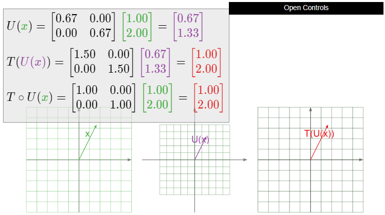
Let \(T\colon\mathbb{R}^2 \to\mathbb{R}^2 \) be dilation by a factor of \(3/2\text{:}\) that is, \(T(x) = 3/2x\). Is \(T\) invertible? If so, what is \(T^{-1}\text{?}\)
Solution
Let \(U\colon\mathbb{R}^2 \to\mathbb{R}^2 \) be dilation by a factor of \(2/3\text{:}\) that is, \(U(x) = 2/3x\). Then
\[ T\circ U(x) = T\biggl(\frac 23x\biggr) = \frac 32\cdot\frac 23x = x \nonumber \]
and
\[ U\circ T(x) = U\biggl(\frac 32x\biggr) = \frac 23\cdot\frac 32x = x. \nonumber \]
Hence \(T\circ U = \text{Id}_{\mathbb{R}^2 }\) and \(U\circ T = \text{Id}_{\mathbb{R}^2 }\text{,}\) so \(T\) is invertible, with inverse \(U\). In other words, shrinking by a factor of \(2/3\) undoes stretching by a factor of 3/2.
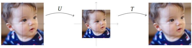
Figure \(\PageIndex{1}\)
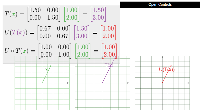
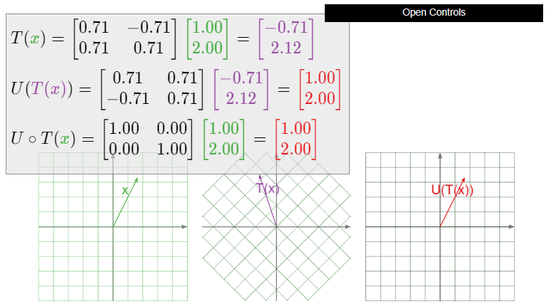
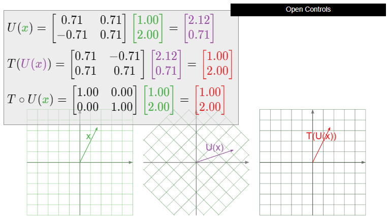
Let \(T\colon\mathbb{R}^2 \to\mathbb{R}^2 \) be counterclockwise rotation by \(45^\circ\). Is \(T\) invertible? If so, what is \(T^{-1}\text{?}\)
Solution
Let \(U\colon\mathbb{R}^2 \to\mathbb{R}^2 \) be clockwise rotation by \(45^\circ\). Then \(T\circ U\) first rotates clockwise by \(45^\circ\text{,}\) then counterclockwise by \(45^\circ\text{,}\) so the composition rotates by zero degrees: it is the identity transformation. Likewise, \(U\circ T\) first rotates counterclockwise, then clockwise by the same amount, so it is the identity transformation. In other words, clockwise rotation by \(45^\circ\) undoes counterclockwise rotation by \(45^\circ\).

Figure \(\PageIndex{4}\)
Let \(T\colon\mathbb{R}^2 \to\mathbb{R}^2 \) be the reflection over the \(y\)-axis. Is \(T\) invertible? If so, what is \(T^{-1}\text{?}\)
Solution
The transformation \(T\) is invertible; in fact, it is equal to its own inverse. Reflecting a vector \(x\) over the \(y\)-axis twice brings the vector back to where it started, so \(T\circ T = \text{Id}_{\mathbb{R}^2 }\).

Figure \(\PageIndex{7}\)

Let \(T\colon\mathbb{R}^3 \to\mathbb{R}^3 \) be the projection onto the \(xy\)-plane, introduced in Example 3.1.3 in Section 3.1. Is \(T\) invertible?
Solution
The transformation \(T\) is not invertible. Every vector on the \(z\)-axis projects onto the zero vector, so there is no way to undo what \(T\) did: the inverse transformation would not know which vector on the \(z\)-axis it should send the zero vector to. More formally, suppose there were a transformation \(U\colon\mathbb{R}^3 \to\mathbb{R}^3 \) such that \(U\circ T = \text{Id}_{\mathbb{R}^3 }\). Then
\[ 0 = U\circ T(0) = U(T(0)) = U(0) \nonumber \]
and
\[ \left(\begin{array}{c}0\\0\\1\end{array}\right) = U\circ T\left(\begin{array}{c}0\\0\\1\end{array}\right) = U\left(T\left(\begin{array}{c}0\\0\\1\end{array}\right)\right) = U(0). \nonumber \]
But \(U(0)\) is as single vector in \(\mathbb{R}^3 \text{,}\) so it cannot be equal to \(0\) and to \((0, 0, 1)\) at the same time.

- A transformation \(T\colon\mathbb{R}^n \to\mathbb{R}^n \) is invertible if and only if it is both one-to-one and onto.
- If \(T\) is already known to be invertible, then \(U\colon\mathbb{R}^n \to\mathbb{R}^n \) is the inverse of \(T\) provided that either \(T\circ U = \text{Id}_{\mathbb{R}^n }\) or \(U\circ T = \text{Id}_{\mathbb{R}^n }\text{:}\) it is only necessary to verify one.
- Proof
-
To say that \(T\) is one-to-one and onto means that \(T(x)=b\) has exactly one solution for every \(b\) in \(\mathbb{R}^n \).
Suppose that \(T\) is invertible. Then \(T(x)=b\) always has the unique solution \(x = T^{-1}(b)\text{:}\) indeed, applying \(T^{-1}\) to both sides of \(T(x)=b\) gives
\[ x = T^{-1}(T(x)) = T^{-1}(b), \nonumber \]
and applying \(T\) to both sides of \(x = T^{-1}(b)\) gives
\[ T(x) = T(T^{-1}(b)) = b. \nonumber \]
Conversely, suppose that \(T\) is one-to-one and onto. Let \(b\) be a vector in \(\mathbb{R}^n \text{,}\) and let \(x = U(b)\) be the unique solution of \(T(x)=b\). Then \(U\) defines a transformation from \(\mathbb{R}^n \) to \(\mathbb{R}^n \). For any \(x\) in \(\mathbb{R}^n \text{,}\) we have \(U(T(x)) = x\text{,}\) because \(x\) is the unique solution of the equation \(T(x) = b\) for \(b = T(x)\). For any \(b\) in \(\mathbb{R}^n \text{,}\) we have \(T(U(b)) = b\text{,}\) because \(x = U(b)\) is the unique solution of \(T(x)=b\). Therefore, \(U\) is the inverse of \(T\text{,}\) and \(T\) is invertible.
Suppose now that \(T\) is an invertible transformation, and that \(U\) is another transformation such that \(T\circ U = \text{Id}_{\mathbb{R}^n }\). We must show that \(U = T^{-1}\text{,}\) i.e., that \(U\circ T = \text{Id}_{\mathbb{R}^n }\). We compose both sides of the equality \(T\circ U = \text{Id}_{\mathbb{R}^n }\) on the left by \(T^{-1}\) and on the right by \(T\) to obtain
\[ T^{-1}\circ T\circ U\circ T = T^{-1}\circ\text{Id}_{\mathbb{R}^n }\circ T. \nonumber \]
We have \(T^{-1}\circ T = \text{Id}_{\mathbb{R}^n }\) and \(\text{Id}_{\mathbb{R}^n }\circ U = U\text{,}\) so the left side of the above equation is \(U\circ T\). Likewise, \(\text{Id}_{\mathbb{R}^n }\circ T = T\) and \(T^{-1}\circ T = \text{Id}_{\mathbb{R}^n }\text{,}\) so our equality simplifies to \(U\circ T = \text{Id}_{\mathbb{R}^n }\text{,}\) as desired.
If instead we had assumed only that \(U\circ T = \text{Id}_{\mathbb{R}^n }\text{,}\) then the proof that \(T\circ U = \text{Id}_{\mathbb{R}^n }\) proceeds similarly.
It makes sense in the above Definition \(\PageIndex{3}\) to define the inverse of a transformation \(T\colon\mathbb{R}^n \to\mathbb{R}^m \text{,}\) for \(m\neq n\text{,}\) to be a transformation \(U\colon\mathbb{R}^m \to\mathbb{R}^n \) such that \(T\circ U = \text{Id}_{\mathbb{R}^m }\) and \(U\circ T = \text{Id}_{\mathbb{R}^n }\). In fact, there exist invertible transformations \(T\colon\mathbb{R}^n \to\mathbb{R}^m \) for any \(m\) and \(n\text{,}\) but they are not linear, or even continuous.
If \(T\) is a linear transformation, then it can only be invertible when \(m = n\text{,}\) i.e., when its domain is equal to its codomain. Indeed, if \(T\colon\mathbb{R}^n \to\mathbb{R}^m \) is one-to-one, then \(n\leq m\) by Note 3.2.1 in Section 3.2, and if \(T\) is onto, then \(m\leq n\) by Note 3.2.2 in Section 3.2. Therefore, when discussing invertibility we restrict ourselves to the case \(m=n\).
Find an invertible (non-linear) transformation \(T\colon\mathbb{R}^2 \to\mathbb{R}\).
As you might expect, the matrix for the inverse of a linear transformation is the inverse of the matrix for the transformation, as the following theorem asserts.
Let \(T\colon\mathbb{R}^n \to\mathbb{R}^n \) be a linear transformation with standard matrix \(A\). Then \(T\) is invertible if and only if \(A\) is invertible, in which case \(T^{-1}\) is linear with standard matrix \(A^{-1}\).
- Proof
-
Suppose that \(T\) is invertible. Let \(U\colon\mathbb{R}^n \to\mathbb{R}^n \) be the inverse of \(T\). We claim that \(U\) is linear. We need to check the defining properties, Definition 3.3.1, in Section 3.3. Let \(u,v\) be vectors in \(\mathbb{R}^n \). Then
\[ u + v = T(U(u)) + T(U(v)) = T(U(u) + U(v)) \nonumber \]
by linearity of \(T\). Applying \(U\) to both sides gives
\[ U(u + v) = U\bigl(T(U(u) + U(v))\bigr) = U(u) + U(v). \nonumber \]
Let \(c\) be a scalar. Then
\[ cu = cT(U(u)) = T(cU(u)) \nonumber \]
by linearity of \(T\). Applying \(U\) to both sides gives
\[ U(cu) = U\bigl(T(cU(u))\bigr) = cU(u). \nonumber \]
Since \(U\) satisfies the defining properties, Definition 3.3.1, in Section 3.3, it is a linear transformation.
Now that we know that \(U\) is linear, we know that it has a standard matrix \(B\). By the compatibility of matrix multiplication and composition, Theorem 3.4.1 in Section 3.4, the matrix for \(T\circ U\) is \(AB\). But \(T\circ U\) is the identity transformation \(\text{Id}_{\mathbb{R}^n },\) and the standard matrix for \(\text{Id}_{\mathbb{R}^n }\) is \(I_n\text{,}\) so \(AB = I_n\). One shows similarly that \(BA = I_n\). Hence \(A\) is invertible and \(B = A^{-1}\).
Conversely, suppose that \(A\) is invertible. Let \(B = A^{-1}\text{,}\) and define \(U\colon\mathbb{R}^n \to\mathbb{R}^n \) by \(U(x) = Bx\). By the compatibility of matrix multiplication and composition, Theorem 3.4.1 in Section 3.4, the matrix for \(T\circ U\) is \(AB = I_n\text{,}\) and the matrix for \(U\circ T\) is \(BA = I_n\). Therefore,
\[ T\circ U(x) = ABx = I_nx = x \quad\text{and}\quad U\circ T(x) = BAx = I_nx = x, \nonumber \]
which shows that \(T\) is invertible with inverse transformation \(U\).
Let \(T\colon\mathbb{R}^2 \to\mathbb{R}^2 \) be dilation by a factor of \(3/2\text{:}\) that is, \(T(x) = 3/2x\). Is \(T\) invertible? If so, what is \(T^{-1}\text{?}\)
Solution
In Example 3.1.5 in Section 3.1 we showed that the matrix for \(T\) is
\[ A = \left(\begin{array}{cc}3/2&0\\0&3/2\end{array}\right). \nonumber \]
The determinant of \(A\) is \(9/4\neq 0\text{,}\) so \(A\) is invertible with inverse
\[ A^{-1} = \frac 1{9/4}\left(\begin{array}{cc}3/2&0\\0&3/2\end{array}\right) = \left(\begin{array}{cc}2/3&0\\0&2/3\end{array}\right). \nonumber \]
By the Theorem \(\PageIndex{3}\), \(T\) is invertible, and its inverse is the matrix transformation for \(A^{-1}\text{:}\)
\[ T^{-1}(x) = \left(\begin{array}{cc}2/3&0\\0&2/3\end{array}\right)x. \nonumber \]
We recognize this as a dilation by a factor of \(2/3\).
Let \(T\colon\mathbb{R}^2 \to\mathbb{R}^2 \) be counterclockwise rotation by \(45^\circ\). Is \(T\) invertible? If so, what is \(T^{-1}\text{?}\)
Solution
In Example 3.3.8 in Section 3.3, we showed that the standard matrix for the counterclockwise rotation of the plane by an angle of \(\theta\) is
\[ \left(\begin{array}{cc}\cos\theta &-\sin\theta \\ \sin\theta &\cos\theta\end{array}\right). \nonumber \]
Therefore, the standard matrix \(A\) for \(T\) is
\[ A = \frac 1{\sqrt 2}\left(\begin{array}{cc}1&-1\\1&1\end{array}\right), \nonumber \]
where we have used the trigonometric identities
\[ \cos(45^\circ) = \frac 1{\sqrt2} \qquad \sin(45^\circ) = \frac 1{\sqrt2}. \nonumber \]
The determinant of \(A\) is
\[ \det(A) = \frac 1{\sqrt2}\cdot\frac 1{\sqrt2} - \frac 1{\sqrt2}\frac{-1}{\sqrt2} = \frac 12 + \frac 12 = 1, \nonumber \]
so the inverse is
\[ A^{-1} = \frac 1{\sqrt2}\left(\begin{array}{cc}1&1\\-1&1\end{array}\right). \nonumber \]
By the Theorem \(\PageIndex{3}\), \(T\) is invertible, and its inverse is the matrix transformation for \(A^{-1}\text{:}\)
\[ T^{-1}(x) = \frac 1{\sqrt2}\left(\begin{array}{cc}1&1\\-1&1\end{array}\right)x. \nonumber \]
We recognize this as a clockwise rotation by \(45^\circ\text{,}\) using the trigonometric identities
\[ \cos(-45^\circ) = \frac 1{\sqrt2} \qquad \sin(-45^\circ) = -\frac 1{\sqrt2}. \nonumber \]
Let \(T\colon\mathbb{R}^2 \to\mathbb{R}^2 \) be the reflection over the \(y\)-axis. Is \(T\) invertible? If so, what is \(T^{-1}\text{?}\)
Solution
In Example 3.1.4 in Section 3.1 we showed that the matrix for \(T\) is
\[ A = \left(\begin{array}{cc}-1&0\\0&1\end{array}\right). \nonumber \]
This matrix has determinant \(-1\text{,}\) so it is invertible, with inverse
\[ A^{-1} = -\left(\begin{array}{cc}1&0\\0&-1\end{array}\right) = \left(\begin{array}{cc}-1&0\\0&1\end{array}\right) = A. \nonumber \]
By the Theorem \(\PageIndex{3}\), \(T\) is invertible, and it is equal to its own inverse: \(T^{-1} = T\). This is another way of saying that a reflection “undoes” itself.