
6.4: Orthogonal Sets
- Page ID
- 70215

- Understand which is the best method to use to compute an orthogonal projection in a given situation.
- Recipes: an orthonormal set from an orthogonal set, Projection Formula, B-coordinates when B is an orthogonal set, Gram–Schmidt process.
- Vocabulary words: orthogonal set, orthonormal set.
In this section, we give a formula for orthogonal projection that is considerably simpler than the one in Section 6.3, in that it does not require row reduction or matrix inversion. However, this formula, called the Projection Formula, only works in the presence of an orthogonal basis. We will also present the Gram–Schmidt process for turning an arbitrary basis into an orthogonal one.
Orthogonal Sets and the Projection Formula
Computations involving projections tend to be much easier in the presence of an orthogonal set of vectors.
A set of nonzero vectors \(\{u_1,\: u_2,\cdots ,u_m\}\) is called orthogonal if \(u_i\cdot u_j=0\) whenever \(i\neq j\). It is orthonormal if it is orthogonal, and in addition \(u_i\cdot u_i=1\) for all \(i=1,\: 2,\cdots ,m\).
In other words, a set of vectors is orthogonal if different vectors in the set are perpendicular to each other. An orthonormal set is an orthogonal set of unit vectors, Definition 6.1.3 in Section 6.1.
The standard coordinate vectors in \(\mathbb{R}^n\) always form an orthonormal set. For instance, in \(\mathbb{R}^3\) we check that
\[\left(\begin{array}{c}1\\0\\0\end{array}\right)\cdot\left(\begin{array}{c}0\\1\\0\end{array}\right)=0\quad\left(\begin{array}{c}1\\0\\0\end{array}\right)\cdot\left(\begin{array}{c}0\\0\\1\end{array}\right)=0\quad\left(\begin{array}{c}0\\1\\0\end{array}\right)\cdot\left(\begin{array}{c}0\\0\\1\end{array}\right)=0.\nonumber\]
Since \(e_i\cdot e_i=1\) for all \(i=1,\: 2,\:3\), this shows that \(\{e_1,\: e_2,\: e_3\}\) is orthonormal.
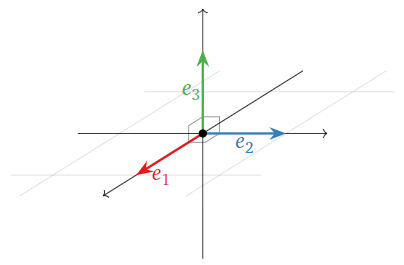
Figure \(\PageIndex{1}\)
Is this set orthogonal? Is it orthonormal?
\[\mathcal{B}=\left\{\left(\begin{array}{c}1\\1\\1\end{array}\right),\left(\begin{array}{c}1\\-2\\1\end{array}\right),\left(\begin{array}{c}1\\0\\-1\end{array}\right)\right\}\nonumber\]
Solution
We check that
\[\left(\begin{array}{c}1\\1\\1\end{array}\right)\cdot\left(\begin{array}{c}1\\-2\\1\end{array}\right)=0\quad\left(\begin{array}{c}1\\1\\1\end{array}\right)\cdot\left(\begin{array}{c}1\\0\\-1\end{array}\right)=0\quad\left(\begin{array}{c}1\\-2\\1\end{array}\right)\cdot\left(\begin{array}{c}1\\0\\-1\end{array}\right)=0.\nonumber\]
Therefore, \(\mathcal{B}\) is orthogonal.
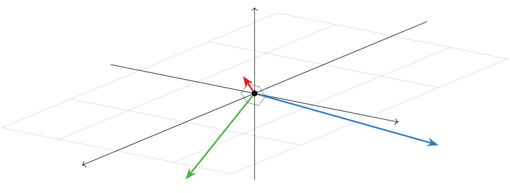
Figure \(\PageIndex{2}\)
The set \(\mathcal{B}\) is not orthonormal because, for instance,
\[\left(\begin{array}{c}1\\1\\1\end{array}\right)\cdot\left(\begin{array}{c}1\\1\\1\end{array}\right)=3\neq 1.\nonumber\]
However, we can make it orthonormal by replacing each vector by the unit vector in the direction of, Fact 6.1.3 in Section 6.1, each vector:
\[\left\{\frac{1}{\sqrt{3}}\left(\begin{array}{c}1\\1\\1\end{array}\right),\:\frac{1}{\sqrt{6}}\left(\begin{array}{c}1\\-2\\1\end{array}\right),\:\frac{1}{\sqrt{2}}\left(\begin{array}{c}1\\0\\-1\end{array}\right)\right\}\nonumber\]
is orthonormal.
We saw in the previous example that it is easy to produce an orthonormal set of vectors from an orthogonal one by replacing each vector with the unit vector in the same direction.
If \(\{v_1,\: v_2,\cdots ,v_m\}\) is an orthogonal set of vectors, then
\[\left\{\frac{v_1}{||v_1||},\:\frac{v_2}{||v_2||},\cdots ,\frac{v_m}{||v_m||}\right\}\nonumber\]
is an orthonormal set.
Let \(a,\:b\) be scalars, and let
\[u_1=\left(\begin{array}{c}a\\b\end{array}\right)\quad u_2=\left(\begin{array}{c}-b\\a\end{array}\right).\nonumber\]
Is \(\mathcal{B}=\{u_1,\: u_2\}\) orthogonal?
Solution
We only have to check that
\[\left(\begin{array}{c}a\\b\end{array}\right)\cdot\left(\begin{array}{c}-b\\a\end{array}\right)=-ab+ab=0.\nonumber\]
Therefore, \(\{u_1,\:u_2\}\) is orthogonal, unless \(a=b=0\).
Is this set orthogonal?
\[\mathcal{B}=\left\{\left(\begin{array}{c}1\\1\\1\end{array}\right),\:\left(\begin{array}{c}1\\-2\\1\end{array}\right),\:\left(\begin{array}{c}1\\-1\\-1\end{array}\right)\right\}\nonumber\]
Solution
This set is not orthogonal because
\[\left(\begin{array}{c}1\\1\\1\end{array}\right)\cdot\left(\begin{array}{c}1\\-1\\-1\end{array}\right)=1-1-1=-1\neq 0.\nonumber\]
We will see how to product an orthogonal set from \(\mathcal{B}\) in the subsection: The Gram-Schmidt Process.
A nice property enjoyed by orthogonal sets is that they are automatically linearly independent.
An orthogonal set is linearly independent. Therefore, it is a basis for its span.
- Proof
-
Suppose that \(\{u_1,\: u_2,\cdots ,u_m\}\) is orthogonal. We need to show that the equation
\[c_1u_1+c_2u_2+\cdots +c_mu_m=0\nonumber\]
has only the trivial solution \(c_1=c_2=\cdots =c_m=0\). Taking the dot product of both sides of this equation with u1 gives
\[\begin{aligned} 0=u_1\cdot 0&=u_1\cdot(c_1u_1+c_2u_2+\cdots +c_mu_m) \\ &=c_1(u_1\cdot u_1)+c_2(u_1\cdot u_2)+\cdots +c_m(u_1\cdot u_m) \\ &=c_1(u_1\cdot u_1)\end{aligned}\]
because \(u_1\cdot u_i=0\) for \(i>1\). Since \(u\neq 0\) we have \(u_1\cdot u_1\neq 0\), so \(c_1=0\). Similarly, taking the dot product with \(u_i\) shows that each \(c_i=0\), as desired.
One advantage of working with orthogonal sets is that it gives a simple formula for the orthogonal projection, Definition 6.3.2 in Section 6.3, of a vector.
Let \(W\) be a subspace of \(\mathbb{R}^n\), and let \(\{u_1,\:u_2,\cdots ,u_m\}\) be an orthogonal basis for \(W\). Then for any vector \(x\) in \(\mathbb{R}^n\), the orthogonal projection of \(x\) onto \(W\) is given by the formula
\[x_{W}=\frac{x\cdot u_1}{u_1\cdot u_1}u_1+\frac{x\cdot u_2}{u_2\cdot u_2}u_2+\cdots +\frac{x\cdot u_m}{u_m\cdot u_m}u_m.\nonumber\]
- Proof
-
Let
\[y=\frac{x\cdot u_1}{u_1\cdot u_1}u_1+\frac{x\cdot u_2}{u_2\cdot u_2}u_2+\cdots +\frac{x\cdot u_m}{u_m\cdot u_m}u_m.\nonumber\]
This vector is contained in \(W\) because it is a linear combination of \(u_1,\: u_2,\cdots ,u_m\). Hence we just need to show that \(x−y\) is in \(W^{\perp}\), i.e., that \(u_i\cdot (x−y)=0\) for each \(i=1,\: 2,\cdots ,m\). For \(u_1\), we have
\[\begin{aligned}u_1\cdot (x-y)&=u_1\cdot\left(x-\frac{x\cdot u_1}{u_1\cdot u_1}u_1-\frac{x\cdot u_2}{u_2\cdot u_2}u_2-\cdots -\frac{x\cdot u_m}{u_m\cdot u_m}u_m\right) \\ &=u_1\cdot x-\frac{x\cdot u_1}{u_1\cdot u_1}(u_1\cdot u_1)-0-\cdots -0 \\ &=0.\end{aligned}\]
A similar calculation shows that \(u_i\cdot (x−y)=0\) for each \(i\), so \(x−y\) is in \(W^{\perp}\), as desired.
If \(\{u_1,\: u_2,\cdots ,u_m\}\) is an orthonormal basis for \(W\), then the denominators \(u_i\cdot u_i=1\) go away, so the projection formula becomes even simpler:
\[x_{W}=(x\cdot u_1)u_1+(x\cdot u_2)u_2+\cdots +(x\cdot u_m)u_m.\nonumber\]
Suppose that \(L=\text{Span}\{u\}\) is a line. The set \(\{u\}\) is an orthogonal basis for \(L\), so the Projection Formula says that for any vector \(x\), we have
\[x_{L}=\frac{x\cdot u}{u\cdot u}u,\nonumber\]
as in Example 6.3.7 in Section 6.3. See also Example 6.3.8 in Section 6.3 and Example 6.3.9 in Section 6.3.
Suppose that \(\{u_1,\: u_2,\cdots ,u_m\}\) is an orthogonal basis for a subspace \(W\), and let \(L_i=\text{Span}\{u_i\}\) for each \(i=1,\: 2,\cdots ,m\). Then we see that for any vector x, we have
\[\begin{aligned}x_{W}&=\frac{x\cdot u_1}{u_1\cdot u_1}u_2+\frac{x\cdot u_2}{u_2\cdot u_2}u_2+\cdots +\frac{x\cdot u_m}{u_m\cdot u_m}u_m \\ &=x_{L_{1}}+x_{L_{2}}+\cdots+x_{L_{m}}\end{aligned}\]
In other words, for an orthogonal basis, the projection of \(x\) onto \(W\) is the sum of the projections onto the lines spanned by the basis vectors. In this sense, projection onto a line is the most important example of an orthogonal projection.
Continuing with Example 6.3.1 in Section 6.3 and Example 6.3.10 in Section 6.3, use the projection formula, Theorem \(\PageIndex{1}\) to compute the orthogonal projection of a vector onto the \(xy\)-plane in \(\mathbb{R}^{3}\).
Solution
A basis for the \(xy\)-plane is given by the two standard coordinate vectors
\[e_1=\left(\begin{array}{c}1\\0\\0\end{array}\right)\quad e_2=\left(\begin{array}{c}0\\1\\0\end{array}\right).\nonumber\]
The set \(\{e_1,\:e_2\}\) is orthogonal, so for any vector \(x=(x_1,\:x_2,\:x_3)\), we have
\[x_{W}=\frac{x\cdot e_1}{e_1\cdot e_1}e_1+\frac{x\cdot e_2}{e_2\cdot e_2}e_2=x_1e_1+x_2e_2=\left(\begin{array}{c}x_1\\x_2\\0\end{array}\right).\nonumber\]
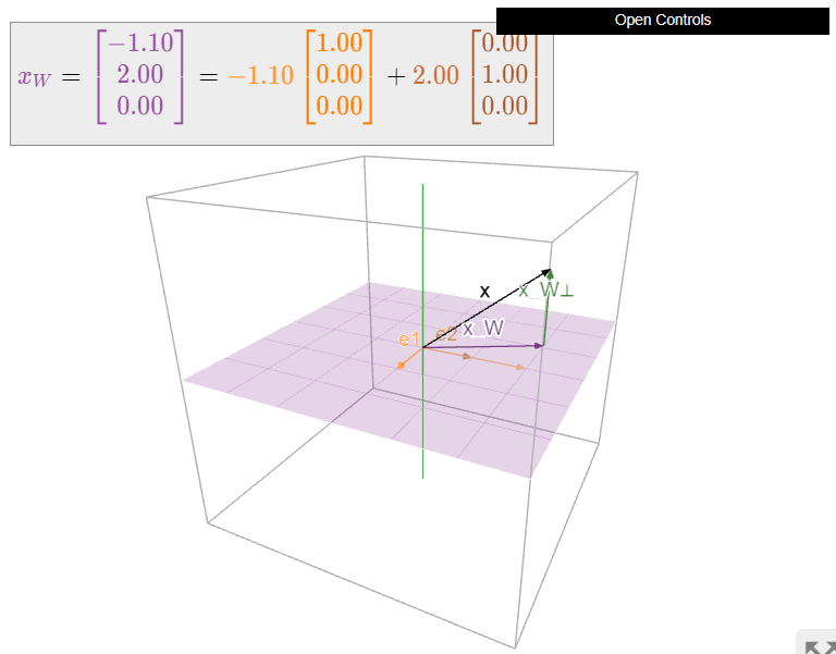
Figure \(\PageIndex{3}\): Orthogonal projection of a vector onto the \(xy\)-plane in \(\mathbb{R}^3\). Note that \(x_{W}\) is the sum of the projections of \(x\) onto the \(e_1\)- and \(e_2\)-coordinate axes (shown in orange and brown, respectively).
Let
\[W=\text{Span}\left\{\left(\begin{array}{c}1\\0\\-1\end{array}\right),\left(\begin{array}{c}1\\1\\1\end{array}\right)\right\}\quad x=\left(\begin{array}{c}2\\3\\-2\end{array}\right).\nonumber\]
Find \(x_{W}\) and \(x_{W^{\perp}}\).
Solution
The vectors
\[u_1=\left(\begin{array}{c}1\\0\\-1\end{array}\right)\quad u_2=\left(\begin{array}{c}1\\1\\1\end{array}\right)\nonumber\]
are orthogonal, so we can use the Projection Formula:
\[x_{W}=\frac{x\cdot u_1}{u_1\cdot u_1}u_1+\frac{x\cdot u_2}{u_2\cdot u_2}u_2=\frac{4}{2}\left(\begin{array}{c}1\\0\\-1\end{array}\right)+\frac{3}{3}\left(\begin{array}{c}1\\1\\1\end{array}\right)=\left(\begin{array}{c}3\\1\\-1\end{array}\right).\nonumber\]
Then we have
\[x_{W^{\perp}}=x-x_{W}=\left(\begin{array}{c}-1\\2\\-1\end{array}\right).\nonumber\]
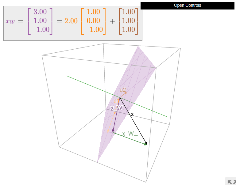
Figure \(\PageIndex{4}\): Orthogonal projection of a vector onto the plane \(W\). Note that \(x_W\) is the sum of the projections of \(x\) onto the lines spanned by \(u_1\) and \(u_2\) (shown in orange and brown, respectively).
Let
\[W=\text{Span}\left\{\left(\begin{array}{c}1\\0\\-1\\0\end{array}\right),\left(\begin{array}{c}0\\1\\0\\-1\end{array}\right),\left(\begin{array}{c}1\\1\\1\\1\end{array}\right)\right\}\quad x=\left(\begin{array}{c}0\\1\\3\\4\end{array}\right).\nonumber\]
Compute \(x_{W}\), and find the distance from \(x\) to \(W\).
Solution
The vectors
\[u_1=\left(\begin{array}{c}1\\0\\-1\\0\end{array}\right)\quad u_2=\left(\begin{array}{c}0\\1\\0\\-1\end{array}\right)\quad u_3=\left(\begin{array}{c}1\\1\\1\\1\end{array}\right)\nonumber\]
are orthogonal, so we can use the Projection Formula:
\[\begin{aligned} x_{W}&=\frac{x\cdot u_1}{u_1\cdot u_1}u_1+\frac{x\cdot u_2}{u_2\cdot u_2}u_2+\frac{x\dot u_3}{u_3\cdot u_3}u_3 \\ &=\frac{-3}{2}\left(\begin{array}{c}1\\0\\-1\\0\end{array}\right)+\frac{-3}{2}\left(\begin{array}{c}0\\1\\0\\-1\end{array}\right)+\frac{8}{4}\left(\begin{array}{c}1\\1\\1\\1\end{array}\right)=\frac{1}{2}\left(\begin{array}{c}1\\1\\7\\7\end{array}\right) \\ x_{W^{\perp}}&=x-x_{W}=\frac{1}{2}\left(\begin{array}{c}-1\\1\\-1\\1\end{array}\right).\end{aligned}\]
The distance from \(x\) to \(W\) is
\[||x_{W^{\perp}}||=\frac{1}{2}\sqrt{1+1+1+1}=1.\nonumber\]
Now let \(W\) be a subspace of \(\mathbb{R}^n\) with orthogonal basis \(\mathcal{B}=\{v_1,\: v_2,\cdots ,v_m\}\), and let \(x\) be a vector in \(W\). Then \(x=x_{W}\), so by the projection formula, Theorem \(\PageIndex{1}\), we have
\[x=x_{W}=\frac{x\cdot u_1}{u_1\cdot u_1}u_1+\frac{x\cdot u_2}{u_2\cdot u_2}u_2+\cdots +\frac{x\cdot u_m}{u_m\cdot u_m}u_m.\nonumber\]
This gives us a way of expressing \(x\) as a linear combination of the basis vectors in \(\mathcal{B}\): we have computed the \(\mathcal{B}\)-coordinates, Definition 2.8.1 in Section 2.8, of \(x\) without row reducing!
Let \(W\) be a subspace of \(\mathbb{R}^n\) with orthogonal basis \(\mathcal{B}=\{v_1,\: v_2,\cdots ,v_m\}\) and let \(x\) be a vector in \(W\). Then
\[[x]_{\mathcal{B}}=\left(\frac{x\cdot u_1}{u_1\cdot u_1},\:\frac{x\cdot u_2}{u_2\cdot u_2},\cdots ,\frac{x\cdot u_m}{u_m\cdot u_m}\right).\nonumber\]
As with orthogonal projections, if \(\{u_1,\: u_2,\cdots ,u_m\}\) is an orthonormal basis of \(W\), then the formula is even simpler:
\[[x]_{\mathcal{B}}=\left(x\cdot u_1,\: x\cdot u_2,\cdots ,x\cdot u_m\right).\nonumber\]
Find the \(\mathcal{B}\)-coordinates of \(x\), where
\[\mathcal{B}=\left\{\left(\begin{array}{c}1\\2\end{array}\right),\left(\begin{array}{c}-4\\2\end{array}\right)\right\}\quad x=\left(\begin{array}{c}0\\3\end{array}\right).\nonumber\]
Solution
Since
\[u_1=\left(\begin{array}{c}1\\2\end{array}\right)\quad u_2=\left(\begin{array}{c}-4\\2\end{array}\right)\nonumber\]
form an orthogonal basis of \(\mathbb{R}^2\), we have
\[[x]_{\mathcal{B}}=\left(\frac{x\cdot u_1}{u_1\cdot u_1},\frac{x\cdot u_2}{u_2\cdot u_2}\right)=\left(\frac{3\cdot 2}{1^2+2^2},\frac{3\cdot 2}{(-4)^2+2^2}\right)=\left(\frac{6}{5},\frac{3}{10}\right).\nonumber\]
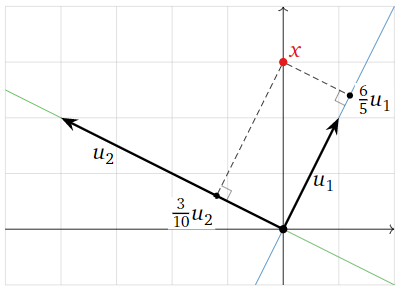
Figure \(\PageIndex{5}\)
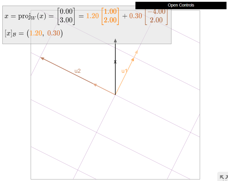
Figure \(\PageIndex{6}\): Computing \(\mathcal{B}\)-coordinates using the Projection Formula.
The following example shows that the Projection Formula does in fact require an orthogonal basis.
Consider the basis \(\mathcal{B}=\{v_1,\: v_2\}\) of \(\mathbb{R}^2\), where
\[v_1=\left(\begin{array}{c}2\\-1/2\end{array}\right)\quad v_2=\left(\begin{array}{c}1\\2\end{array}\right).\nonumber\]
This is not orthogonal because \(v_1\cdot v_2=2−1=1\neq 0\). Let \(x=\left(\begin{array}{c}1\\1\end{array}\right)\). Let us try to compute \(x=x_{\mathbb{R}^{2}}\) using the Projection Formula with respect to the basis \(\mathcal{B}\):
\[x_{\mathbb{R}^{2}}=\color{Green}{\frac{x\cdot v_1}{v_1\cdot v_1}v_1}\color{black}{+}\color{Purple}{\frac{x\cdot v_2}{v_2\cdot v_2}v_2}\color{black}{=}\color{Green}{\frac{3/2}{17/4}\left(\begin{array}{c}2\\-1/2\end{array}\right)}\color{black}{+}\color{Purple}{\frac{3}{5}\left(\begin{array}{c}1\\2\end{array}\right)}\color{black}{=\left(\begin{array}{c}111/85\\ 87/85\end{array}\right)\neq x.}\nonumber\]
Since \(x=x_{\mathbb{R}^{2}}\), we see that the Projection Formula does not compute the orthogonal projection in this case. Geometrically, the projections of \(x\) onto the lines spanned by \(v_1\) and \(v_2\) do not sum to \(x\), as we can see from the picture.
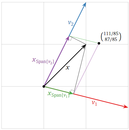
Figure \(\PageIndex{7}\)
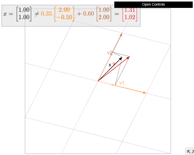
Figure \(\PageIndex{8}\): When \(v_1\) and \(v_2\) are not orthogonal, then \(x_{\mathbb{R}^{2}}=x\) is not necessarily equal to the sum (red) of the projections (orange and brown) of \(x\) onto the lines spanned by \(v_1\) and \(v_2\).
You need an orthogonal basis to use the Projection Formula.
The Gram-Schmidt Process
We saw in the previous subsection that orthogonal projections and \(\mathcal{B}\)-coordinates are much easier to compute in the presence of an orthogonal basis for a subspace. In this subsection, we give a method, called the Gram–Schmidt Process, for computing an orthogonal basis of a subspace.
Let \(v_1,\: v_2,\cdots ,v_m\) be a basis for a subspace \(W\) of \(\mathbb{R}^{n}\). Define:
- \(u_1=v_1\)
- \(u_2=(v_2)_{\text{Span}\{u_1\}^{\perp}}\qquad\qquad =v_2-\frac{v_2\cdot u_1}{u_1\cdot u_1}u_1\)
- \(u_3=(v_3)_{\text{Span}\{u_1,u_2\}^{\perp}}\qquad\quad\; =v_3-\frac{v_3\cdot u_1}{u_1\cdot u_1}u_1-\frac{v_3\cdot u_2}{u_2\cdot u_2}u_2\)
\(\quad\vdots\)
- \(u_m=(v_m)_{\text{Span}\{u_1,u_2,\cdots ,u_{m-1}\}^{\perp}}=v_m-\sum\limits_{i=1}^{m-1}\frac{v_m\cdot u_i}{u_i\cdot u_i}u_i\).
Then \(\{u_1,\: u_2,\cdots ,u_m\}\) is an orthogonal basis for the same subspace \(W\).
- Proof
-
First we claim that each \(u_i\) is in \(W\), and in fact that \(u_i\) is in \(\text{Span}\{v_1,\: v_2,\cdots ,v_i\}\). Clearly \(u_1=v_1\) is in \(\text{Span}\{v_1\}\). Then \(u_2\) is a linear combination of \(u_1\) and \(v_2\), which are both in \(\text{Span}\{v_1,\: v_2\}\), so \(u_2\) is in \(\text{Span}\{v_1,\:v_2\}\) as well. Similarly, \(u_3\) is a linear combination of \(u_1,\: u_2\), and \(v_3\), which are all in \(\text{Span}\{v_1,\: v_2,\: v_3\}\), so \(u_3\) is in \(\text{Span}\{v_1,\: v_2,\: v_3\}\). Continuing in this way, we see that each \(u_i\) is in \(\text{Span}\{v_1,\: v_2,\cdots ,v_i\}\).
Now we claim that \(\{u_1,\: u_2,\cdots ,u_m\}\) is an orthogonal set. Let \(1\leq i < j\leq m\). Then \(u_j=(v_j)_{\text{Span}\{u_1,\:u_2,\cdots ,u_{j−1}\}^{\perp}}\), so by definition \(u_j\) is orthogonal to every vector in \(\text{Span}\{u_1,\:u_2,\cdots ,u_{j−1}\}\). In particular, \(u_j\) is orthogonal to \(u_i\).
We still have to prove that each \(u_i\) is nonzero. Clearly \(u_1=v_1\neq 0\). Suppose that \(u_i=0\). Then \((v_i)_{\text{Span}\{u_1,\:u_2,\cdots,u_{i−1}\}^{\perp}}=0\), which means that \(v_i\) is in \(\text{Span}\{u_1,\:u_2,\cdots ,u_{i−1}\}\). But each \(u_1,\: u_2,\cdots ,u_{i−1}\) is in \(\text{Span}\{v_1,\:v_2,\cdots ,v_{i−1}\}\) by the first paragraph, so \(v_i\) is in \(\text{Span}\{v_1,\: v_2,\cdots ,v_{i−1}\}\). This contradicts the increasing span criterion Theorem 2.5.2 in Section 2.5; therefore, \(u_i\) must be nonzero.
The previous two paragraphs justify the use of the projection formula, Theorem \(\PageIndex{1}\), in the equalities
\[(v_i)_{\text{Span}\{u_1,\:u_2,\cdots ,u_{i-1}\}^{\perp}}=v_i-(v_i)_{\text{Span}\{u_1,\:u_2,\cdots ,u_{i-1}\}}=v_i-\sum\limits_{j=1}^{i-1}\frac{v_i\cdot u_j}{u_j\cdot u_j}u_j\nonumber\]
in the statement of the theorem.
Since \(\{u_1,\: u_2,\cdots ,u_m\}\) is an orthogonal set, it is linearly independent. Thus it is a set of \(m\) linearly independent vectors in \(W\), so it is a basis for \(W\) by the basis theorem, Theorem 2.7.3 in Section 2.7. Similarly, for every \(i\), we saw that the set \(\{u_1,\: u_2,\cdots ,u_i\}\) is contained in the \(i\)-dimensional subspace \(\text{Span}\{v_1,\:v_2,\cdots ,v_i\}\), so \(\{u_1,\:u_2,\cdots ,u_i\}\) is an orthogonal basis for \(\text{Span}\{v_1,\:v_2,\cdots ,v_i\}\).
Find an orthogonal basis \(\{u_1,\:u_2\}\) for \(W=\text{Span}\{v_1,\:v_2\}\), where
\[v_1=\left(\begin{array}{c}1\\1\\0\end{array}\right)\quad v_2=\left(\begin{array}{c}1\\1\\1\end{array}\right).\nonumber\]
Solution
We run Gram–Schmidt: first take \(u_1=v_1\), then
\[u_2=v_2-\frac{v_2\cdot u_1}{u_1\cdot u_1}u_1=\left(\begin{array}{c}1\\1\\1\end{array}\right)-\frac{2}{2}\left(\begin{array}{c}1\\1\\0\end{array}\right)=\left(\begin{array}{c}0\\0\\1\end{array}\right).\nonumber\]
Then \(\{u_1,\:u_2\}\) is an orthogonal basis for \(W\): indeed, it is clear that \(u_1\cdot u_2=0\).
Geometrically, we are simply replacing \(v_2\) with the part of \(v_2\) that is perpendicular to line \(L_1=\text{Span}\{v_1\}\):
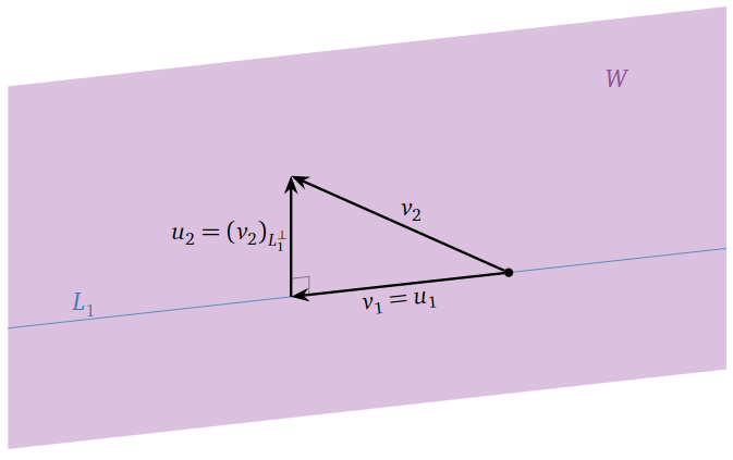
Figure \(\PageIndex{9}\)
Find an orthogonal basis \(\{u_1,\: u_2,\:u_3\}\) for \(W=\text{Span}\{v_1,\:v_2,\:v_3\}=\mathbb{R}^3\), where
\[v_1=\left(\begin{array}{c}1\\1\\0\end{array}\right)\quad v_2=\left(\begin{array}{c}1\\1\\1\end{array}\right)\quad v_3=\left(\begin{array}{c}3\\1\\1\end{array}\right).\nonumber\]
Solution
We run Gram-Schmidt:
- \(u_1=v_1=\left(\begin{array}{c}1\\1\\0\end{array}\right)\)
- \(u_2=v_2=\frac{v_2\cdot u_1}{u_1\cdot u_1}u_1=\left(\begin{array}{c}1\\1\\1\end{array}\right)-\frac{2}{2}\left(\begin{array}{c}1\\1\\0\end{array}\right)=\left(\begin{array}{c}0\\0\\1\end{array}\right)\)
- \(\begin{aligned}u_3&=v_3-\frac{v_3\cdot u_1}{u_1\cdot u_1}u_1-\frac{v_3\cdot u_2}{u_2\cdot u_2}u_2 \\ &=\left(\begin{array}{c}3\\1\\1\end{array}\right)-\frac{4}{2}\left(\begin{array}{c}1\\1\\0\end{array}\right)-\frac{1}{1}\left(\begin{array}{c}0\\0\\1\end{array}\right)=\left(\begin{array}{c}1\\-1\\0\end{array}\right).\end{aligned}\)
Then \(\{u_1,\:u_2,\:u_3\}\) is an orthogonal basis for \(W\): indeed, we have
\[u_1\cdot u_2=0\quad u_1\cdot u_3=0\quad u_2\cdot u_3=0.\nonumber\]
Geometrically, once we have \(u_1\) and \(u_2\), we replace \(v_3\) by the part that is orthogonal to \(W_2=\text{Span}\{u_1,\:u_2\}=\text{Span}\{v_1,\:v_2\}\):
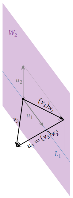
Figure \(\PageIndex{10}\)
Find an orthogonal basis \(\{u_1,\:u_2,\:u_3\}\) for \(W=\text{Span}\{v_1,\:v_2,\:v_3\}\), where
\[v_1=\left(\begin{array}{c}1\\1\\1\\1\end{array}\right)\quad v_2=\left(\begin{array}{c}-1\\4\\4\\-1\end{array}\right)\quad v_3=\left(\begin{array}{c}4\\-2\\-2\\0\end{array}\right).\nonumber\]
Solution
We run Gram–Schmidt:
- \(u_1=v_1=\left(\begin{array}{c}1\\1\\1\\1\end{array}\right)\)
- \(u_2=v_2-\frac{v_2\cdot u_1}{u_1\cdot u_1}u_1=\left(\begin{array}{c}-1\\4\\4\\-1\end{array}\right)-\frac{6}{4}\left(\begin{array}{c}1\\1\\1\\1\end{array}\right)=\left(\begin{array}{c}-5/2\\5/2\\5/2\\-5/2\end{array}\right)\)
- \(\begin{aligned}u_3&=v_3-\frac{v_3\cdot u_1}{u_1\cdot u_1}u_1-\frac{v_3\cdot u_2}{u_2\cdot u_2}u_2 \\ &=\left(\begin{array}{c}4\\-2\\-2\\0\end{array}\right)-\frac{0}{24}\left(\begin{array}{c}1\\1\\1\\1\end{array}\right)-\frac{-20}{25}\left(\begin{array}{c}-5/2\\5/2\\5/2\\-5/2\end{array}\right)=\left(\begin{array}{c}2\\0\\0\\-2\end{array}\right).\end{aligned}\)
Then \(\{u_1,\:u_2,\:u_3\}\) is an orthogonal basis for \(W\).
We saw in the proof of the Gram–Schmidt Process that for every \(i\) between \(1\) and \(m\), the set \(\{u_1,\:u_2,\cdots ,u_i\}\) is a an orthogonal basis for \(\text{Span}\{v_1,\:v_2,\cdots ,v_i\}\).
If we had started with a spanning set \(\{v_1,\:v_2,\cdots ,v_m\}\) which is linearly dependent, then for some \(i\), the vector \(v_i\) is in \(\text{Span}\{v_1,\:v_2,\cdots ,v_{i−1}\}\) by the increasing span criterion, Theorem 2.5.2 in Section 2.5. Hence
\[0=(v_i)_{\text{Span}\{v_1,\:v_2,\cdots ,v_{i-1}\}^{\perp}}=(v_i)_{\text{Span}\{u_1,\:u_2,\cdots u_{i-1}\}^{\perp}}=u_i.\nonumber\]
You can use the Gram–Schmidt Process to produce an orthogonal basis from any spanning set: if some \(u_i=0\), just throw away \(u_i\) and \(v_i\), and continue.