
6.1: Dot Products and Orthogonality
- Page ID
- 70212

- Understand the relationship between the dot product, length, and distance.
- Understand the relationship between the dot product and orthogonality.
- Vocabulary words: dot product, length, distance, unit vector, unit vector in the direction of \(x\).
- Essential vocabulary word: orthogonal.
In this chapter, it will be necessary to find the closest point on a subspace to a given point, like so:
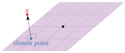
Figure \(\PageIndex{1}\)
The closest point has the property that the difference between the two points is orthogonal, or perpendicular, to the subspace. For this reason, we need to develop notions of orthogonality, length, and distance.
The Dot Product
The basic construction in this section is the dot product, which measures angles between vectors and computes the length of a vector.
The dot product of two vectors \(x,y\) in \(\mathbb{R}^n \) is
\[ x\cdot y = \left(\begin{array}{c}x_1\\x_2\\ \vdots\\x_n\end{array}\right) \cdot \left(\begin{array}{c}y_1\\y_2\\ \vdots\\ y_n\end{array}\right) \;=\; x_1y_1 + x_2y_2 + \cdots + x_ny_n. \nonumber \]
Thinking of \(x,y\) as column vectors, this is the same as \(x^Ty\).
For example,
\[ \left(\begin{array}{c}1\\2\\3\end{array}\right)\cdot\left(\begin{array}{c}4\\5\\6\end{array}\right) = \left(\begin{array}{ccc}1&2&3\end{array}\right)\left(\begin{array}{c}4\\5\\6\end{array}\right) = 1\cdot 4 + 2\cdot 5 + 3\cdot 6 = 32. \nonumber \]
Notice that the dot product of two vectors is a scalar.
You can do arithmetic with dot products mostly as usual, as long as you remember you can only dot two vectors together, and that the result is a scalar.
Let \(x,y,z\) be vectors in \(\mathbb{R}^n \) and let \(c\) be a scalar.
- Commutativity: \(x\cdot y = y \cdot x\).
- Distributivity with addition: \((x + y)\cdot z = x\cdot z+y\cdot z\).
- Distributivity with scalar multiplication: \((cx)\cdot y = c(x\cdot y)\).
The dot product of a vector with itself is an important special case:
\[ \left(\begin{array}{c}x_1\\x_2\\ \vdots\\x_n\end{array}\right) \cdot\left(\begin{array}{c}x_1\\x_2\\ \vdots\\x_n\end{array}\right) = x_1^2 + x_2^2 + \cdots + x_n^2. \nonumber \]
Therefore, for any vector \(x\text{,}\) we have:
- \(x\cdot x \geq 0\)
- \(x\cdot x = 0 \iff x = 0.\)
This leads to a good definition of length.
The length of a vector \(x\) in \(\mathbb{R}^n \) is the number
\[ \|x\| = \sqrt{x\cdot x} = \sqrt{x_1^2 + x_2^2 + \cdots + x_n^2}. \nonumber \]
It is easy to see why this is true for vectors in \(\mathbb{R}^2 \text{,}\) by the Pythagorean theorem.
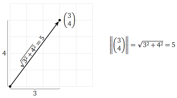
Figure \(\PageIndex{1}\)
For vectors in \(\mathbb{R}^3 \text{,}\) one can check that \(\|x\|\) really is the length of \(x\text{,}\) although now this requires two applications of the Pythagorean theorem.
Note that the length of a vector is the length of the arrow; if we think in terms of points, then the length is its distance from the origin.
Suppose that \(\|x\| = 2,\;\|y\|=3,\) and \(x\cdot y = -4\). What is \(\|2x + 3y\|\text{?}\)
Solution
We compute
\[ \begin{split} \|2x+3y\|^2 &= (2x+3y)\cdot(2x+3y) \\ &= 4x\cdot x + 6x\cdot y + 6x\cdot y + 9y\cdot y \\ &= 4\|x\|^2 + 9\|y\|^2 + 12x\cdot y \\ &= 4\cdot 4 + 9\cdot 9 - 12\cdot 4 = 49. \end{split} \nonumber \]
Hence \(\|2x+3y\| = \sqrt{49} = 7.\)
If \(x\) is a vector and \(c\) is a scalar, then \(\|cx\|=|c|\cdot\|x\|.\)
This says that scaling a vector by \(c\) scales its length by \(|c|\). For example,
\[ \left\|\left(\begin{array}{c}6\\8\end{array}\right)\right\| = \left\|2\left(\begin{array}{c}3\\4\end{array}\right)\right\| = 2\left\|\left(\begin{array}{c}3\\4\end{array}\right)\right\| = 10. \nonumber \]
Now that we have a good notion of length, we can define the distance between points in \(\mathbb{R}^n \). Recall that the difference between two points \(x,y\) is naturally a vector, namely, the vector \(y-x\) pointing from \(x\) to \(y\).
The distance between two points \(x,y\) in \(\mathbb{R}^n \) is the length of the vector from, Note 2.1.2 in Section 2.1, \(x\) to \(y\text{:}\)
\[ \text{dist}(x,y) = \|y-x\|. \nonumber \]
Find the distance from \((1,2)\) to \((4,4)\).
Solution
Let \(x=(1,2)\) and \(y=(4,4)\). Then
\[ \text{dist}(x,y) = \|y-x\| = \left\|\left(\begin{array}{c}3\\2\end{array}\right)\right\| = \sqrt{3^2+2^2} = \sqrt{13}. \nonumber \]
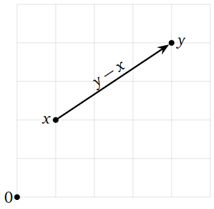
Figure \(\PageIndex{2}\)
Vectors with length \(1\) are very common in applications, so we give them a name.
A unit vector is a vector \(x\) with length \(\|x\| = \sqrt{x\cdot x} =1\).
The standard coordinate vectors, Note 3.3.2 in Section 3.3, \(e_1,e_2,e_3,\ldots\) are unit vectors:
\[ \|e_1\| = \left\|\left(\begin{array}{c}1\\0\\0\end{array}\right)\right\| = \sqrt{1^2 + 0^2 + 0^2} = 1. \nonumber \]
For any nonzero vector \(x\text{,}\) there is a unique unit vector pointing in the same direction. It is obtained by dividing by the length of \(x\).
Let \(x\) be a nonzero vector in \(\mathbb{R}^n \). The unit vector in the direction of \(x\) is the vector \(x/\|x\|\).
This is in fact a unit vector (noting that \(\|x\|\) is a positive number, so \(\bigl|1/\|x\|\bigr| = 1/\|x\|\)):
\[ \left\|\frac{x}{\|x\|}\right\| = \frac 1{\|x\|}\|x\| = 1. \nonumber \]
What is the unit vector \(u\) in the direction of \(x = \left(\begin{array}{c}3\\4\end{array}\right)\text{?}\)
Solution
We divide by the length of \(x\text{:}\)
\[ u = \frac{x}{\|x\|} = \frac 1{\sqrt{3^2+4^2}}\left(\begin{array}{c}3\\4\end{array}\right) = \frac{1}{5}\left(\begin{array}{c}3\\4\end{array}\right) = \left(\begin{array}{c}3/5\\4/5\end{array}\right). \nonumber \]
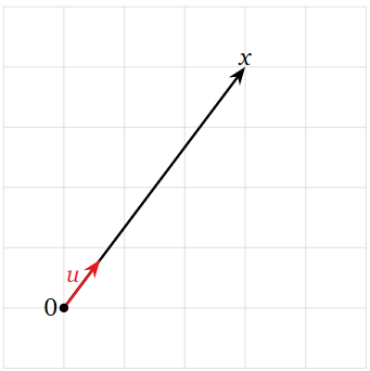
Figure \(\PageIndex{3}\)
Orthogonal Vectors
In this section, we show how the dot product can be used to define orthogonality, i.e., when two vectors are perpendicular to each other.
Two vectors \(x,y\) in \(\mathbb{R}^n \) are orthogonal or perpendicular if \(x\cdot y = 0\).
Notation: \(x\perp y\) means \(x\cdot y = 0\).
Since \(0 \cdot x = 0\) for any vector \(x\text{,}\) the zero vector is orthogonal to every vector in \(\mathbb{R}^n \).
We motivate the above definition using the law of cosines in \(\mathbb{R}^2 \). In our language, the law of cosines asserts that if \(x,y\) are two nonzero vectors, and if \(\alpha>0\) is the angle between them, then
\[ \|y-x\|^2 = \|x\|^2 + \|y\|^2 - 2\|x\|\,\|y\|\cos\alpha. \nonumber \]
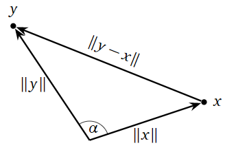
Figure \(\PageIndex{4}\)
In particular, \(\alpha=90^\circ\) if and only if \(\cos(\alpha)=0\text{,}\) which happens if and only if \(\|y-x\|^2 = \|x\|^2+\|y\|^2\). Therefore,
\[ \begin{split} \text{$x$ and $y$ are perpendicular} \amp\iff \|x\|^2 + \|y\|^2 = \|y-x\|^2 \\ \amp\iff x\cdot x + y\cdot y = (y-x)\cdot(y-x) \\ \amp\iff x\cdot x + y\cdot y = y\cdot y + x\cdot x -2x\cdot y \\ \amp\iff x\cdot y = 0. \end{split} \nonumber \]
To reiterate:
\[ x\perp y \quad\iff\quad x\cdot y = 0 \quad\iff\quad \|y-x\|^2 = \|x\|^2 + \|y\|^2. \nonumber \]
Find all vectors orthogonal to \(v = \left(\begin{array}{c}1\\1\\-1\end{array}\right).\)
Solution
We have to find all vectors \(x\) such that \(x\cdot v = 0\). This means solving the equation
\[ 0 = x\cdot v = \left(\begin{array}{c}x_1\\x_2\\x_3\end{array}\right)\cdot\left(\begin{array}{c}1\\1\\-1\end{array}\right) = x_1 + x_2 - x_3. \nonumber \]
The parametric form for the solution set is \(x_1 = -x_2 + x_3\text{,}\) so the parametric vector form of the general solution is
\[ x = \left(\begin{array}{c}x_1\\x_2\\x_3\end{array}\right) = x_2\left(\begin{array}{c}-1\\1\\0\end{array}\right) + x_3\left(\begin{array}{c}1\\0\\1\end{array}\right). \nonumber \]
Therefore, the answer is the plane
\[ \text{Span}\left\{\left(\begin{array}{c}-1\\1\\0\end{array}\right),\;\left(\begin{array}{c}1\\0\\1\end{array}\right)\right\}. \nonumber \]
For instance,
\[\left(\begin{array}{c}-1\\1\\0\end{array}\right)\perp\left(\begin{array}{c}1\\1\\-1\end{array}\right)\quad\text{because}\quad \left(\begin{array}{c}-1\\1\\0\end{array}\right)\cdot\left(\begin{array}{c}1\\1\\-1\end{array}\right) = 0\text{.} \nonumber \]
Find all vectors orthogonal to both \(v = \left(\begin{array}{c}1\\1\\-1\end{array}\right)\) and \(w = \left(\begin{array}{c}1\\1\\1\end{array}\right)\).
Solution
We have to solve the system of two homogeneous equations
\[\begin{aligned}0&=x\cdot v=\left(\begin{array}{c}x_1\\x_2\\x_3\end{array}\right)\cdot\left(\begin{array}{c}1\\1\\-1\end{array}\right)=x_1+x_2-x_3 \\ 0&=x\cdot w=\left(\begin{array}{c}x_1\\x_2\\x_3\end{array}\right)\cdot\left(\begin{array}{c}1\\1\\1\end{array}\right)=x_1+x_2+x_3.\end{aligned}\]
In matrix form:
\[ \left(\begin{array}{ccc}1&1&-1\\1&1&1\end{array}\right) \;\xrightarrow{\text{RREF}}\;\left(\begin{array}{ccc}1&1&0\\0&0&1\end{array}\right). \nonumber \]
The parametric vector form of the solution set is
\[ \left(\begin{array}{c}x_1\\x_2\\x_3\end{array}\right) = x_2\left(\begin{array}{c}-1\\1\\0\end{array}\right). \nonumber \]
Therefore, the answer is the line
\[ \text{Span}\left\{\left(\begin{array}{c}-1\\1\\0\end{array}\right)\right\}. \nonumber \]
For instance,
\[ \left(\begin{array}{c}-1\\1\\0\end{array}\right)\cdot\left(\begin{array}{c}1\\1\\-1\end{array}\right) = 0 \quad\text{and}\quad \left(\begin{array}{c}-1\\1\\0\end{array}\right)\cdot\left(\begin{array}{c}1\\1\\1\end{array}\right) = 0. \nonumber \]
More generally, the law of cosines gives a formula for the angle \(\alpha\) between two nonzero vectors:
\[ \begin{split} 2\|x\|\|y\|\cos(\alpha) \amp= \|x\|^2 + \|y\|^2 - \|y-x\|^2 \\ \amp= x\cdot x + y\cdot y - (y-x)\cdot (y-x) \\ \amp= x\cdot x + y\cdot y - y\cdot y - x\cdot x + 2x\cdot y \\ \amp= 2x\cdot y \\ \amp\quad\implies \alpha = \cos^{-1}\left(\frac{x\cdot y}{\|x\|\|y\|}\right). \end{split} \nonumber \]
In higher dimensions, we take this to be the definition of the angle between \(x\) and \(y\).