
17.1: Singular Value Decomposition
- Page ID
- 2095

Suppose
\[L:V \overset{Linear}{\rightarrow} W\, .\]
It is unlikely that \(\dim V:=n=m=:\dim W\) so the \(m\times n\) matrix \(M\) of \(L\) in bases for \(V\) and \(W\) will not be square. Therefore there is no eigenvalue problem we can use to uncover a preferred basis. However, if the vector spaces \(V\) and \(W\) both have inner products, there does exist an analog of the eigenvalue problem, namely the singular values of \(L\).
Before giving the details of the powerful technique known as the singular value decomposition, we note that it is an excellent example of what Eugene Wigner called the "Unreasonable Effectiveness of Mathematics'':
There is a story about two friends who were classmates in high school, talking about their jobs. One of them became a statistician and was working on population trends. He showed a reprint to his former classmate. The reprint started, as usual with the Gaussian distribution and the statistician explained to his former classmate the meaning of the symbols for the actual population and so on. His classmate was a bit incredulous and was not quite sure whether the statistician was pulling his leg. ``How can you know that?'' was his query. "And what is this symbol here?'' "Oh,'' said the statistician, this is "\(\pi\).'' "And what is that?'' "The ratio of the circumference of the circle to its diameter.'' "Well, now you are pushing your joke too far,'' said the classmate, "surely the population has nothing to do with the circumference of the circle.''
-- Eugene Wigner, Commun. Pure and Appl. Math. {\bf XIII}, 1 (1960).
Whenever we mathematically model a system, any "canonical quantities'' (those on which we can all agree and do not depend on any choices we make for calculating them) will correspond to important features of the system. For examples, the eigenvalues of the eigenvector equation you found in review question 1, chapter 12 encode the notes and harmonics that a guitar string can play! Singular values appear in many linear algebra applications, especially those involving very large data sets such as statistics and signal processing.
Let us focus on the \(m\times n\) matrix \(M\) of a linear transformation \(L:V\to W\) written in orthonormal bases for the input and outputs of \(L\) (notice, the existence of these othonormal bases is predicated on having inner products for \(V\) and \(W\)). Even though the matrix \(M\) is not square, both the matrices \(M M^{T}\) and \(M^{T} M\) are square and symmetric! In terms of linear transformations \(M^{T}\) is the matrix of a linear transformation
$$L^{*}: W \overset{Linear}{\rightarrow} V\, .\]
Thus \(LL^{*}:W\to W\) and \(L^{*}L:V\to V\) and both have eigenvalue problems. Moreover, as we learned in chapter 15, both \(L^{*}L\) and \(LL^{*}\) have orthonormal bases of eigenvectors, and both \(MM^{T}\) and \(M^{T}M\) can be diagonalized.
Next, let us make a simplifying assumption, namely \(ker L=\{0\}\). This is not necessary, but will make some of our computations simpler. Now suppose we have found an orthonormal basis \((u_{1},\ldots , u_{n})\) for \(V\) composed of eigenvectors for \(L^{*}L\):
\[
L^{*}L u_{i}= \lambda_{i} u_{i}\, .
\]
Hence, multiplying by \(L\),
\[
L L^{*} L u_{i} = \lambda_{i} L u_{i}\, .
\]
\(\textit{i.e.}\), \(L u_{i}\) is an eigenvector of \(L L^{*}\). The vectors \((Lu_{1},\ldots, Lu_{n})\) are linearly independent, because \(ker L=\{0\}\) (this is where we use our simplifying assumption, but you can try and extend our analysis to the case where it no longer holds). Lets compute the angles between, and lengths of these vectors:
For that we express the vectors \(u_{i}\) in the bases used to compute the matrix \(M\) of \(L\). Denoting these column vectors by \(U_{i}\) we then compute
\[
(MU_{i})\cdot (MU_{j})=U_{i}^{T} M^{T} M U_{j} = \lambda_{j} \, U_{i}^{T} U_{j}=\lambda_{j} \, U_{i}\cdot U_{j}= \lambda_{j} \delta_{ij}\, .
\]
Hence we see that vectors \((Lu_{1},\ldots, Lu_{n})\) are orthogonal but not orthonormal. Moreover, the length of \(Lu_{i}\) is \(\lambda_{i}\).
Thus, normalizing lengths, we have that
\[
\left(\frac{Lu_{1}}{\sqrt{\lambda_{1}}},\ldots,\frac{Lu_{n}}{\sqrt{\lambda_{n}}}\right)
\]
are orthonormal and linearly independent. However, since \(ker L=\{0\}\) we have \(\dim L(V)=\dim V\) and in turn \(\dim V\leq \dim W\), so \(n\leq m\). This means that although the above set of \(n\) vectors in \(W\) are orthonormal and linearly independent, they cannot be a basis for \(W\). However, they are a subset of the eigenvectors of \(LL^{*}\). Hence an orthonormal basis of eigenvectors of \(LL^{*}\) looks like
\[
O'=\left(\frac{Lu_{1}}{\sqrt{\lambda_{1}}},\ldots,\frac{Lu_{n}}{\sqrt{\lambda_{n}}},v_{m+1},\ldots,v_{m}\right)=:(v_{1},\ldots,v_{m})\, .
\]
Now lets compute the matrix of \(L\) with respect to the orthonormal basis \(O=(u_{1},\ldots,u_{n})\) for \(V\) and the orthonormal basis \(O'=(v_{1},\ldots,v_{m})\) for \(W\). As usual, our starting point is the computation of \(L\) acting on the input basis vectors:
\begin{eqnarray*}
\big(Lu_{1},\ldots, Lu_{n}\big)&=&
\big(\sqrt{\lambda_{1}}\, v_{1},\ldots,\sqrt{\lambda_{n}}\, v_{n}\big)\\&=&\big(v_{1},\ldots,v_{m}\big)
\begin{pmatrix}
\sqrt{\lambda_{1}}&0&\cdots&0\\
0&\sqrt{\lambda_{2}}&\cdots&0\\
{\vdots}&\vdots&\ddots&\vdots\\
0&0&\cdots&\sqrt{\lambda_{n}}\\
0 & 0& \cdots &0\\
{\vdots}&\vdots&&\vdots\\
0 & 0& \cdots &0
\end{pmatrix}\, .
\end{eqnarray*}
The result is very close to diagonalization; the numbers \(\sqrt{\lambda_{i}}\) along the leading diagonal are called the singular values of \(L\).
Example \(\PageIndex{1}\):
Let the matrix of a linear transformation be
\[
M=\begin{pmatrix}
\frac{1}{2}&\frac{1}{2}\\-1&1\\-\frac{1}{2}&-\frac{1}{2}
\end{pmatrix}\, .
\]
Clearly \(ker M=\{0\}\) while
\[
M^{T}M=\begin{pmatrix}\frac{3}{2}&-\frac{1}{2}\\-\frac{1}{2}&\frac{3}{2}\end{pmatrix}
$$
which has eigenvalues and eigenvectors
$$
\lambda=1\, ,\, u_{1}:=\begin{pmatrix}\frac{1}{\sqrt{2}}\\\frac{1}{\sqrt{2}}\end{pmatrix}; \qquad
\lambda=2\, ,\, u_{2}:=\begin{pmatrix}\frac{1}{\sqrt{2}}\\-\frac{1}{\sqrt{2}}\end{pmatrix}\,\, .
$$
so our orthonormal input basis is $$O=\left(\begin{pmatrix}\frac{1}{\sqrt{2}}\\\frac{1}{\sqrt{2}}\end{pmatrix},\begin{pmatrix}\frac{1}{\sqrt{2}}\\-\frac{1}{\sqrt{2}}\end{pmatrix}\right)\, .
$$
These are called the \(\textit{right singular vectors}\) of \(M\). The vectors
$$
M u_{1}= \begin{pmatrix}\frac{1}{\sqrt{2}}\\{\ \ 0}\\-\frac{1}{\sqrt{2}}\end{pmatrix} \mbox{ and }
M u_{2}=\begin{pmatrix}0\\-\sqrt{2}\\0\end{pmatrix}
$$
are eigenvectors of
$$M M^{T}=\begin{pmatrix}\frac{1}{2}&\ 0&\!-\frac{1}{2}\\0&2&0\\-\frac{1}{2}&0&\frac{1}{2}\end{pmatrix}$$
with eigenvalues \(1\) and \(2\), respectively. The third eigenvector (with eigenvalue \(0\)) of \(M\) is
$$v_{3}=\begin{pmatrix}\frac{1}{\sqrt{2}}\\{\ \ 0}\\-\frac{1}{\sqrt{2}}\end{pmatrix}\, .$$
The eigenvectors \(Mu_{1}\) and \(Mu_{2}\) are necessarily orthogonal, dividing them by their lengths we obtain the \(\textit{left singular vectors}\) and in turn our orthonormal output basis
$$
O'=\left(\begin{pmatrix}\frac{1}{\sqrt{2}}\\{\ \ 0}\\-\frac{1}{\sqrt{2}}\end{pmatrix},\begin{pmatrix}0\\-1\\0\end{pmatrix},\begin{pmatrix}\frac{1}{\sqrt{2}}\\{\ \ 0}\\\frac{1}{\sqrt{2}}\end{pmatrix}\right)\, .
$$
The new matrix \(M'\) of the linear transformation given by \(M\) with respect to the bases \(O\) and \(O'\) is
$$
M'=\begin{pmatrix}
1&0\\0&\sqrt{2}\\0&0
\end{pmatrix}\, ,
$$
so the singular values are \(1,\sqrt{2}\).
Finally note that arranging the column vectors of \(O\) and \(O'\) into change of basis matrices
$$
P=\begin{pmatrix}
\frac{1}{\sqrt{2}}&\frac{1}{\sqrt{2}}\\
\frac{1}{\sqrt{2}}&-\frac{1}{\sqrt{2}}
\end{pmatrix}\, ,\qquad
Q=
\begin{pmatrix}
\frac{1}{\sqrt{2}}&0&\frac{1}{\sqrt{2}}\\
{\ \ 0}&-1&0\\
\!-\frac{1}{\sqrt{2}}&0&\frac{1}{\sqrt{2}}
\end{pmatrix}\, ,
$$
we have, as usual,
$$
M'=Q^{-1}MP\, .
\]
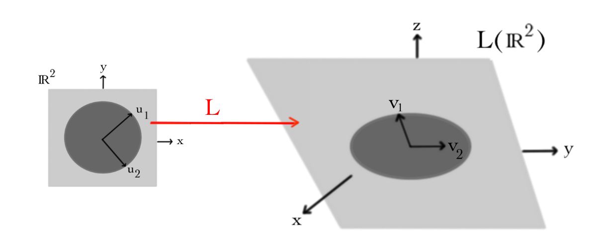
Singular vectors and values have a very nice geometric interpretation: they provide an orthonormal bases for the domain and range of \(L\) and give the factors by which \(L\) stretches the orthonormal input basis vectors. This is depicted below for the example we just computed:
Contributors and Attributions
David Cherney, Tom Denton, and Andrew Waldron (UC Davis)