2.1: Linear Functions

Last updated
Save as PDF

Page ID: 62725

$ \newcommand{\vecs}[1]{\overset { \scriptstyle \rightharpoonup} {\mathbf{#1}} } $ $ \newcommand{\vecd}[1]{\overset{-\!-\!\rightharpoonup}{\vphantom{a}\smash {#1}}} $$\newcommand{\id}{\mathrm{id}}$ $ \newcommand{\Span}{\mathrm{span}}$ $ \newcommand{\kernel}{\mathrm{null}\,}$ $ \newcommand{\range}{\mathrm{range}\,}$ $ \newcommand{\RealPart}{\mathrm{Re}}$ $ \newcommand{\ImaginaryPart}{\mathrm{Im}}$ $ \newcommand{\Argument}{\mathrm{Arg}}$ $ \newcommand{\norm}[1]{\| #1 \|}$ $ \newcommand{\inner}[2]{\langle #1, #2 \rangle}$ $ \newcommand{\Span}{\mathrm{span}}$ $\newcommand{\id}{\mathrm{id}}$ $ \newcommand{\Span}{\mathrm{span}}$ $ \newcommand{\kernel}{\mathrm{null}\,}$ $ \newcommand{\range}{\mathrm{range}\,}$ $ \newcommand{\RealPart}{\mathrm{Re}}$ $ \newcommand{\ImaginaryPart}{\mathrm{Im}}$ $ \newcommand{\Argument}{\mathrm{Arg}}$ $ \newcommand{\norm}[1]{\| #1 \|}$ $ \newcommand{\inner}[2]{\langle #1, #2 \rangle}$ $ \newcommand{\Span}{\mathrm{span}}$$\newcommand{\AA}{\unicode[.8,0]{x212B}}$

In this section, we will discuss linear functions. A linear function is a polynomial with degree 1. In calculus, you will learn how to use lines to approximate more complicated functions in order to better understand their behavior at or near a point. These linear approximations can help us evaluate nearby points on the complicated function more easily and can tell us how quickly the function is changing. Linear approximations can also be used to help us determine the area of irregular shapes.

2.1.1: Properties of Lines

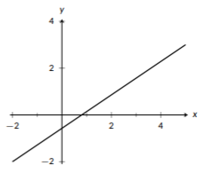
$clipboard_e6723e45dec919edcad5f610f337d25cc.png$

Figure $\PageIndex{1}$: A line with a positive slope.

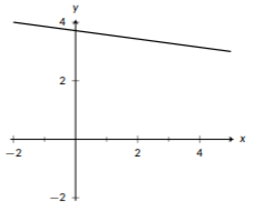
$clipboard_ea44497347beee24c7f7a708f1370cf1b.png$

Figure $\PageIndex{2}$: A line with a negative slope.

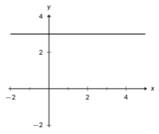
$clipboard_e428b4b1a9e86954c51b52b32d2d55d2d.png$

Figure $\PageIndex{3}$: A line with a slope of $0$.

Every line can be uniquely defined based on two keep features: the slope of the line and a point contained by the line. The slope of the line tells us about its steepness, and the point gives us a place to anchor the line. If the points on a line go up as you move to the right, it has a positive slope, and the bigger the slope is the faster the line increases, or the steeper it is. You can see an example of a line with positive slope in Figure $\PageIndex{1}$. If the points on a line go down as you move to the right, it has a negative slope. A more negative slope indicates that it decreases faster. If the points neither go up nor down as you move to the right, it has a slope of 0, indicating that the line is horizontal.

Visually, it’s straightforward to determine if the slope is positive, negative, or 0. Typically, we need more detailed information and will need to calculate the slope. To do this from a graph, we need to find two points on the line. We’ll call these two points $(x_1,y_1)$ and $(x_2,y_2)$. Notice that each point includes two values, an x-value and a y-value. When you pick two points, you may use any two distinct points you like; no matter what you pick you will always get the same result for the slope. Mathematicians typically use $m$ as the symbol for slope. The formula is:

\[m = \frac{y_1-y_2}{x_1-x_2}\label{formula}\]

The numerator tells us how much change we have in y (vertical change) between the points and the denominator tells us how much change we have in x (horizontal change). Sometimes, you’ll see the formula written like this:

\[m = \frac{\Delta y}{\Delta x}\label{change}\]

The symbol $\Delta$ (the capital Greek letter “delta”) tells us we are looking at change, so $\Delta y$ means change in y and $\Delta x$ means changes in $x$. Formulas $\eqref{formula}$ and $\eqref{change}$ have the same meaning, they just look a little different.

Example $\PageIndex{1}$: Finding Slope

Determine the slope of the line in Figure $\PageIndex{1}$.

Solution

To determine the slope, we will need two points from the graph. Any two points will work, but we will use $(-2,-2)$ and $(5,3)$ since both $x$ and $y$ are integer values at these points. We’ll call $(-2,2)$ our first point; this means $x_1=-2$ and $y_1=-2$. We’ll call $(5,3)$ our second point; this means $x_2=5$ and $y_2=3$. Then, we just need to plug into the formula for slope:

\[\begin{align}\begin{aligned}\begin{split} m= \frac{y_1-y_2}{x_1-x_2} & = \frac{-2-3}{-2-5} \\ & = \frac{-5}{-7} \\ & = \frac{5}{7} \end{split}\end{aligned}\end{align}\] Therefore, the slope of the line in Figure $\PageIndex{1}$ is

\[m=\frac{5}{7}\]

Earlier, we talked about how a line is defined by its slope and a point, but slope itself is determined by two points on the line. This means that we can also uniquely define a line from two points that are on the line. We can take both to find the slope, and then use either of the points as our anchor.

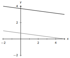
$clipboard_eeeb3188acafe33e5782cb2cec766bad0.png$

Figure $\PageIndex{4}$: Parallel lines.

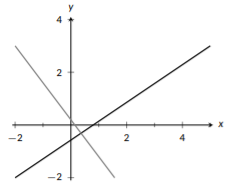
$clipboard_e347c9367ca681d8270b06816be08c14f.png$

Figure $\PageIndex{5}$: Perpendicular lines.

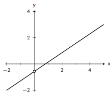
$clipboard_eec9858f984cca046483b76e80d649fd2.png$

Figure $\PageIndex{6}$: The $y$-intercept of a line.

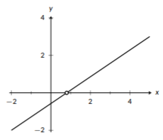
$clipboard_e3b8fad4ecede160ad310b11cbc24683b.png$

Figure $\PageIndex{7}$: The $x$-intercept of a line.

If two lines have the same slope, we say they are parallel. Parallel lines will never intersect each other since they have the same steepness (unless they are really the same line). If two lines are not parallel, they have to intersect at one point. If the lines form a right angle ($90^{\circ}$) when they intersect, they are perpendicular. Like parallel lines where $m_1=m_2$ (the slope of line 1 is the same as the slope of line 2), perpendicular lines also have related slopes. Here, if line 1 and line 2 are perpendicular, $m_1 =-\frac{1}{m_2}$. We could rearrange this equation to solve for $m_2$ and we would get $m_2 = -\frac{1}{m_1}$. Notice that the formula looks the same, except $m_1$ and $m_2$ are swapped. This relationship is described as “negative reciprocal;” negative since the sign is opposite and reciprocal since we invert the relationship. We’ll see this property used in example $\PageIndex{4}$.

When we look at a line, we can use any two points to describe it, but there are two points that mathematicians are more likely to use. The first (and most commonly used) is the y-intercept. This is the point where the line crosses (“intercepts”) the y-axis. Since $x=0$ on the y-axis, this point looks like $(0,y_{int})$. Similarly, the x-intercept is frequently used. The x-intercept is the point where the line crosses the x-axis, so it has $y=0$ and looks like $(x_{int},0)$. These two points are commonly used because they are easier to work with since one of the coordinates is 0.

2.1.2: Expressing Linear Functions

There are two common ways of expressing linear functions, point-slope form and slope-intercept form. As you can probably guess from the names, both of these forms will require that you first know the slope. Slope-intercept form requires knowing the y-intercept of the function, and point-slope form allows you to use any point on the line. It’s good to be comfortable working with both forms and with switching between them because sometimes one form will be more useful than the other. In calculus, point-slope form often comes in handy because we will be looking at lines over a small region that won’t always contain the y-intercept of the line. Slope-intercept form is:

\[\label{eqn:slope_intercept_form} y=mx+b\]

where $m$ is the slope of the function and $b$ is the y-coordinate of the y-intercept. Point-slope form is:

\[\label{eqn:point_slope_form} y-y_1 = m(x-x_1)\]

where $m$ is the slope and $(x_1,y_1)$ is any point on the line. Let’s take a look at an example of how to work with both of these forms.

Example $\PageIndex{2}$: Writing an Equation for a Line

Write the equation for the line that passes through $(2,4)$ and is parallel to $3x+y=6$ in slope-intercept form.

Solution

Let’s analyze the information we so far. First, we know that our line goes through the point $(2,4)$. We know we also need its slope.

We’re told it’s parallel to $3x+y=6$, so it will have the same slope as that line. However, this line isn’t in either of our forms, so it’s not immediately clear what the slope is. We’ll start by putting this line, $3x+y=6$ into slope-intercept form (because it requires less algebra than putting it into point-slope form would). To put it into slope-intercept form, we need to isolate $y$. We’ll do that by subtracting $3x$ from both sides. That gives \[y=6-3x\]

If we rearrange the right side, we get $y=-3x+6$. Now, it’s in slope-intercept form and we can see that the slope is $-3$.

Now, we have the slope of our line, $m=-3$, and a point on our line, $(2,4)$, and our goal is to express the line in slope-intercept form. There’s a slight problem with this- we don’t know the y-intercept. Luckily, we do have enough information to express the line in point-slope form, so we’ll start with that and use algebra to get it into slope-intercept form. In point-slope form, we have: \[y-4=-3(x-2)\]

We’ll use algebra to rewrite this in slope-intercept form (i.e., we’ll isolate y): \[\begin{align}\begin{aligned}\begin{split} y-4 & = -3x+6 \\ y & = -3x+6+4 \\ y & = -3x+10 \end{split}\end{aligned}\end{align}\]

So, in slope-intercept form, the line is $y=-3x+10$. This also tells us that the y-intercept of this line is $(0,10)$. Our final answer, in slope-intercept form, is

\[y=-3x+10\]

This isn’t the only way to answer this question, so let’s try a second method. The two methods will always give you the same result, so it’s entirely a matter of preference when choosing which method to use.

Example $\PageIndex{3}$: Writing an Equation for a Line- A Second Method

Write the equation for the line that passes through $(2,4)$ and is parallel to $3x+y=6$ in slope-intercept form.

Solution

From our previous work on this problem, we know that our line goes through the point $(2,4)$ and that it has a slope of $-3$. We also know that slope-intercept form looks like \[y=mx+b\]

and that this statement holds for every $(x,y)$ pair that are on the line. We know $m$, but we are missing $b$. However, we do know that $(2,4)$ is on the line, so \[y=-3x+b\]

needs to be true for $x=2$ and $y=4$. We’ll substitute these values into our equation and solve for $b$: \[\begin{align}\begin{aligned}\begin{split} 4 & =-3(2)+b\\ 4 & = -6 + b\\ 10 & = b \end{split}\end{aligned}\end{align}\]

Now, we know $b$, so our final answer, in slope-intercept form, is again

Let’s look at one more example, this time working with a perpendicular line.

Example $\PageIndex{4}$: Perpendicular Line

In slope-intercept form, write the equation of a line with a y-intercept of 5 that is perpendicular to $y-4=6(x-2)$.

Solution

Let’s look at the information we have so far. We are told that the line we are interested in has a y-intercept of 5. We know that $x=0$ for the y-intercept, so this really means that the y-intercept is the point $(0,5)$. Next, we know that we are perpendicular to the line $y-4=6(x-2)$. This line is given in point-slope form and has a slope of 6.

The slope of our line has to be $-\frac{1}{6}$ since it’s perpendicular to a line with a slope of 6. Overall, that gives us that the equation of our line, in slope-intercept form, is

\[y=-\frac{1}{6}x+5\]