2.4: Graphs and Graphing

Last updated
Save as PDF

Page ID: 63331

$ \newcommand{\vecs}[1]{\overset { \scriptstyle \rightharpoonup} {\mathbf{#1}} } $ $ \newcommand{\vecd}[1]{\overset{-\!-\!\rightharpoonup}{\vphantom{a}\smash {#1}}} $$\newcommand{\id}{\mathrm{id}}$ $ \newcommand{\Span}{\mathrm{span}}$ $ \newcommand{\kernel}{\mathrm{null}\,}$ $ \newcommand{\range}{\mathrm{range}\,}$ $ \newcommand{\RealPart}{\mathrm{Re}}$ $ \newcommand{\ImaginaryPart}{\mathrm{Im}}$ $ \newcommand{\Argument}{\mathrm{Arg}}$ $ \newcommand{\norm}[1]{\| #1 \|}$ $ \newcommand{\inner}[2]{\langle #1, #2 \rangle}$ $ \newcommand{\Span}{\mathrm{span}}$ $\newcommand{\id}{\mathrm{id}}$ $ \newcommand{\Span}{\mathrm{span}}$ $ \newcommand{\kernel}{\mathrm{null}\,}$ $ \newcommand{\range}{\mathrm{range}\,}$ $ \newcommand{\RealPart}{\mathrm{Re}}$ $ \newcommand{\ImaginaryPart}{\mathrm{Im}}$ $ \newcommand{\Argument}{\mathrm{Arg}}$ $ \newcommand{\norm}[1]{\| #1 \|}$ $ \newcommand{\inner}[2]{\langle #1, #2 \rangle}$ $ \newcommand{\Span}{\mathrm{span}}$$\newcommand{\AA}{\unicode[.8,0]{x212B}}$

In calculus, we will be analyzing graphs to learn more about the functions they represent. It is important that we have a good understanding of the relationship between a function and its graph. Specifically in differential calculus, we will learn to use derivatives (which is a rate of change or the local slope) to determine where a graph is increasing or decreasing. Also, in integral calculus, you might learn how to calculate the work required to pump a fluid, which gives a chance to explore the value of using different locations for the origin, effectively resulting in a shift of the function and its graph.

2.4.1 Graphs of General Functions

Many people take a very tedious approach to graphing; for the domain they are interested in graphing, they take each possible integer value of $x$, evaluate the function for that value, and then graph a single point. After they have graphed several points across the domain, they will “connect the dots.” While this method is reliable, it is time consuming, and can be difficult depending on the function. In this section, we will give an overview of the general shape of common functions and then talk about how these general functions can be shifted, stretched, and flipped in order to quickly sketch related functions. Additionally, we will talk about piecewise functions and how to graph them correctly.

Lines

The quickest way to graph a line is by using a point and the slope. This is largely because both forms, slope-intercept and point-slope, provide you with this information. Start by plotting the point. Then, from that point use the slope to plot a second point. For example, if the slope is $-\frac{2}{3}$, you would start at the initial point, move $3$ units to the right (because the horizontal change is 3), and then move down $2$ units in the y-direction (because the slope is negative and the vertical change is 2). (Note: you can also move vertically and then horizontally, either way gives the same result.) Plot this new point, and then use a straightedge to connect both points. Be sure to continue past each of the points. If the slope is a whole number, move that many units vertically and only one unit to the right to plot your second point.

Example $\PageIndex{1}$: Graphing a Line

Graph the line $y=2x-3$

Solution

Let’s start by identifying the slope and a point. We are in slope-intercept form, so we can see that the slope is $m=2$ and the y-intercept is $(0,-3)$. We’ll starting by plotting a point at $(0,-3)$. Then, we’ll move to the right 1 unit and up 2 units and plot a second point. Then, we use the two points to draw our line. The full process is shown in the following three graphs:

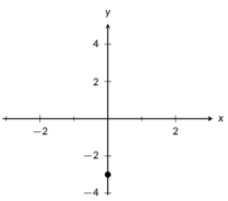
$clipboard_ef8a60f94209297d950c83c236a58f590.png$

Figure $\PageIndex{1}$: Plot the $y$-intercept

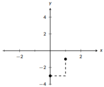
$clipboard_e8da68b92f6fd6855af96765042d286ba.png$

Figure $\PageIndex{2}$: Use the slope to plot a second point

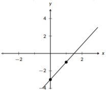
$clipboard_e7603f4d13e2187e9c08958a3d43d12b6.png$

Figure $\PageIndex{3}$: Complete the line

Quadratic Functions

The most basic quadratic function is $f(x)=x^2$.Later, we will discuss how every other quadratic function can be graphed by shifting and stretching this function. The general shape of this function is a “U” and it is symmetric over the y-axis, meaning that the left and right sides of the graph are a reflection of each other. This function grows quickly; this means that as $x$ gets big, $f(x)$ gets big faster than $x$ does. It has no horizontal asymptotes, meaning that as $x$ gets big, $f(x)$ doesn’t level off.

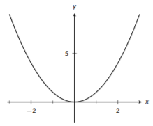
$clipboard_e1f4c290b751dc977869473b659a3909b.png$

Figure $\PageIndex{4}$: The graph of $f(x)=x^{2}$.

Cubic Functions

The most basic cubic function is $f(x)=x^3$. Similarly to the quadratic functions, every other cubic function can be graphed by shifting and stretching this function. This function has rotational symmetry around the origin; if you treat $(0,0)$ like a pivot point and rotate the graph $180^{\circ}$, it will looks exactly the same. For positive values of $x$, this function grows quickly, but for negative values of $x$ it becomes more and more negative. It also has no horizontal asymptotes.

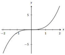
$clipboard_ee04399b88b329174c878980654f77598.png$

Figure $\PageIndex{5}$: The graph of $f(x)=x^{3}$.

Even Polynomials

An even polynomial is any polynomial where every monomial has an even degree. For example, $f(x)=x^6+3x^4-5x^2+7$ is an even polynomial because the degrees are 6, 4, 2, and 0. However, $g(x)=x^4-x^2+x-4$ is not an even polynomial because it has $x$ as a term (and $x$ has degree 1). Even polynomials share features with the basic quadratic function: they are symmetric about the y-axis and both “tails” of the function have the same sign. This means that as $x$ gets very big or very negative, $f(x)$ will have the same sign; either both tails are positive or both tails are negative. This is a key feature of even polynomials. The sign on the highest degree term tells you if both of the tails will be positive or if both will be negative.

A related, but slightly different, type of function is a polynomial of even order, also known as a polynomial of even degree. Here, we only care about the highest degree term being even, so both $f(x)$ and $g(x)$ from above are polynomials of even order. These polynomials don’t have to be symmetric about the y-axis, but they do exhibit the same “end” behavior where either both tails are positive or both tails are negative.

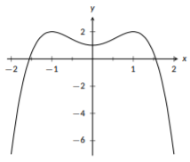
$clipboard_e46a8838ee1b305231c7bc89f233f6fc5.png$

Figure $\PageIndex{6}$: The graph of $f(x)=-x^{4}+2x^{2}+1$, an even polynomial.

Odd Polynomials

An odd polynomial is any polynomial where every monomial has an odd degree. For example, $f(x)=4x^5+2x^3-7x$ is an odd polynomial because the degrees are 5, 3, and 1. However, $g(x)=2x^3+x-7$ is not and odd polynomial because it has $-7$ as a term (and $-7$ has degree 0). Odd polynomials share features with the basic cubic functions: they have rotational symmetry about the origin and the tails have opposite signs. Odd polynomials always have one positive tail and one negative tail.

Again, we have a related type of function, a polynomial of odd order, also known as a polynomial of odd degree. For these polynomials, the highest degree must be odd, but smaller degree terms can be even, as in $h(x)=x^3+2x^2$. These polynomials aren’t all symmetric about the origin, but the tails will have opposite signs.

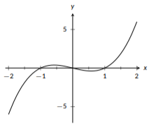
$clipboard_e40ad8d69dee85c7ba8d1d37fdeec0ea0.png$

Figure $\PageIndex{7}$: The graph of $f(x)=x^{3}-x$, an odd polynomial.

Exponential Functions

For a basic exponential function, $f(x)=b^x$, $b$ must be a positive real number with $b\neq 1$. All basic exponential functions with $b>1$ share some key features: they all contain the point $(0,1)$, they all contain the point $(1,b)$, they grow quickly for positive values of $x$, and for negative values of $x$ they get close to $y=0$, the x-axis. A basic exponential function will never cross the x-axis, it will only get closer and closer as $x$ gets more and more negative. This long-term behavior is described as having an horizontal asymptote at $y=0$. When graphing an exponential function, we plot the two key points listed above and use the general shape to guide the rest of our graph.

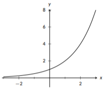
$clipboard_e38e782605d04e49e6721cc30e773b116.png$

Figure $\PageIndex{8}$: The graph of $f(x)-2^{x}$, a basic exponential function.

Logarithmic Functions

Logarithmic functions have the same shape as basic exponential functions, but reflected over the line $y=x$. This means that the key features of functions of the form $f(x)=\log_b{(x)}$ are: they all contain the point $(1,0)$; they all contain the point $(b,1)$; for very small positive values of $x$, $f(x)$ becomes increasingly negative if $b>1$ and increasingly positive if $b<1$; as $x$ becomes very large, so does $f(x)$ if $b>1$ and very negative if $b<1$. It’s important when graphing logarithmic functions to remember that their domain is only $(0,\infty)$; you should graph nothing for negative values of $x$ and nothing for $x=0$. Logarithmic functions have a vertical asymptote at $x=0$, the y-axis. The graph gets very close to this vertical line, but it will never cross it.

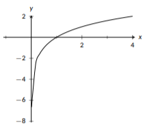
$clipboard_e42ae753574652530e459aef545f74ea9.png$

Figure $\PageIndex{9}$: The graph of $f(x)=\log_{2}(x)$, a basic logarithmic function.

Trigonometric Functions

A key feature of the trigonometric functions $\sin{(x)}$, $\cos{(x)}$, and $\tan{(x)}$ is that all three are periodic functions; they exhibit the same pattern over and over. Additionally, the sine and cosine functions never grow without bound; their $y$ values are always between $-1$ and $1$. The tangent function does grow without bound and has repeat vertical asymptotes. For all three functions, there are key points when $x$ is a multiple of $\pi$, such as $x=\frac{\pi}{2}$, $x=\pi$, $x=\frac{3\pi}{2}$, and $x=2\pi$. Additionally, you might notice that the graphs of sine and cosine are very similar. In fact, if you take the graph of sine and shift it to the left by $\frac{\pi}{2}$ you would get the graph of cosine. In fact, this is a trigonometric identity that can be seen just from the graphs. The graphs of these three functions can be seen below:

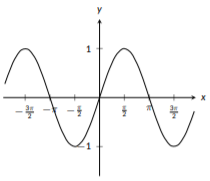
$clipboard_e47d7116d5902be94ae289b51d78a7098.png$

Figure $\PageIndex{10}$: The graph of $f(x)=\sin (x)$

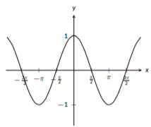
$clipboard_eb1b3ee116d2973fa244ff4bae0bddfb5.png$

Figure $\PageIndex{11}$: The graph of $f(x)=\cos(x)$

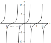
$clipboard_e923ccc4c9db569e934c3271b04d0b59d.png$

Figure $\PageIndex{12}$: The graph of $f(x)=\tan(x)$

2.4.2: Modifying Functions

Now that we’ve seen the shapes of some basic functions like $f(x)=x^2$, let’s talk about how we can use these basic shapes to help graph many functions. We’ll need to be able to identify the base function we are working with and to identify how it’s been modified. We’ll break these down into two main types of modifications: vertical modifications and horizontal modifications. Vertical modifications will, as the name says, will affect the functions vertically, either shifting the function up or down, or stretching or shrinking the function’s height. Similarly, horizontal modifications will affect the function horizontally, shifting it left or right, or stretching or shrinking its “width.”

Vertical Modifications

The first type of vertical modifications we will discuss are shifts, where every point on the functions gets shifted up or down by the same distance. This is one of the easiest modifications to spot; all we have to do is add or subtract a constant to the function. Let’s take a look at an example.

Example $\PageIndex{2}$: Shifting a Function Vertically

Graph the function $f(x)=x^2+3$.

Solution

Here we can see that we have a function with a constant added to it; this tells us that we need to graph $x^2$, but with a vertical shift. The constant, $+3$ tells us that we will take this base function and shift it up $3$ units (if this was $-3$ we would shift the function down by 3 units).

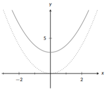
$clipboard_e0b839479f0ed6cdd622c2e2e6e287d39.png$

Figure $\PageIndex{13}$: Vertical Shift

Here, the graph shows both our base function, $x^2$ (dotted) and our desired, shifted function, $f(x)=x^2+3$ (solid). If you take a piece of wire and shape it to match the graph of $x^2$, you can move the wire up 3 units and see that you get exactly the graph of $f(x)=x^2+3$.

Notice that with a vertical shift, the shape of the function does not change at all, only its positioning relative to the x axis changes. With our next modification, vertical stretching and shrinking, we don’t change its positioning, or the shape, but we do change how steep the function is. With vertical stretches, everything on the x-axis is fixed, so the positioning doesn’t change. The shape doesn’t change in the sense that every quadratic will still look like a “U” and every sine or cosine will still look like never-ending waves (similarly for our other functions). So how do we recognize when a function is being stretched or shrunk vertically? We’ll have a base function that is being modified with scalar multiplication, such as $f(x)=3\sin{(x)}$ or $g(t)= -\frac{1}{2} t^3$.Here, if we multiply by a number bigger than 1 or less than $-1$, we will stretch the function and make it steeper. If we multiply it by anything between $-1$ and $1$, it will shrink and get less steep. If we multiply by a negative number, not only is the function being stretched or shrunk, it will also be flipped; everything above the x-axis will be reflected to below the x-axis and everything below will be reflection to above the x-axis.

Example $\PageIndex{3}$: Stretching/Shrinking a Function Vertically

Graph the functions $f(x)=\frac{1}{2} x^3$ and $g(x)=-\frac{1}{2}x^3$.

Solution

For both $f(x)$ and $g(x)$ we have the same base function, $x^3$. Since $f(x)$ is formed by multiplying this by $\frac{1}{2}$, it is being shrunk, but not flipped.

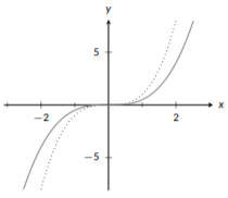
$clipboard_ece9ded63e33073910669fab46d4089d6.png$

Figure $\PageIndex{14}$: Vertical Shrink

Here we can see our base function, $x^3$ (dotted) and $f(x)=\frac{1}{2}x^3$ (solid). You’ll see that the shape and position are still the same, but $f(x)$ stays closer to the x-axis; it does not get tall as quickly as $x^3$ does because we shrunk the graph vertically. Now that we’ve shrunk the graph, flipping it will give us the graph of $g(x)$ (solid):

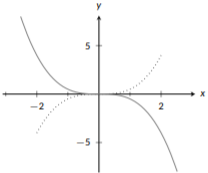
$clipboard_e1b53b463113dc60a9b7a3073027f078e.png$

Figure $\PageIndex{15}$: Vertical Shrink

This graph has both $f(x)$ (dotted) and $g(x)$ (solid); both have the same position and the same steepness, but $g(x)$ is upside-down.

The previous example shows how to shrink and flip a graph. Here, you could do either step first; if you flip and then shrink you would get the exact same result. We recommend making very quick sketches in the margins of your page when dealing with multiple transformations at the same time; it makes it easier for me to make sure we draw the final graph accurately by capturing each stage, however, after practice you may feel comfortable doing both steps at once.

We’ve now seen how we vertical modifications work individually, but what happens when we combine them?

Example $\PageIndex{4}$: Multiple Vertical Modifications

Graph $h(x) = 2\sin{(x)} - 1$.

Solution

First, let’s identify our base function. Here, we are working with $\sin{(x)}$. We see that we are multiplying by 2 and subtracting 1; this tells us we have a vertical stretch and a vertical shift. Which should we do first? The answer comes from our order of operations: multiplication should be done before subtraction. We’ll follow that same rule here by stretching $\sin{(x)}$ and then shifting it. Since we have $2\sin{(x)}$ in our function, we will start by graphing $\sin{(x)}$ (dotted) and then making it twice as “tall” (i.e., twice as far from the x-axis; solid graph).

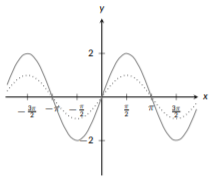
$clipboard_ed9b560570e5d6d4a3644bf2f6ed5c3c1.png$

Figure $\PageIndex{16}$: Sine

Now that we’ve stretched it, we can take care of the addition and shift it down 1 unit:

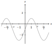
$clipboard_ef399ac9297ad4fdc6a6d7a91f6f3bb5c.png$

Figure $\PageIndex{17}$: Sine shifted

Horizontal Modifications

We can make the same modifications horizontally that we made vertically: stretching, shrinking, and shifting. With vertical modifications, the modifications showed up on the outside of the function, with shifts added to the end and with stretches coming as multiplication out front. With horizontal changes we will work on the inside of the function. For example, if we want to shift the function $f(x)$ 2 units to the left, we would graph $f(x+2)$. This moves the graph of $f$ to the left because, in essence, we always looking at a bigger input than what x really is, e.g., if $x=4$, really we are looking at $f(4+2)=f(6)$. Similarly, if we want to shift $f$ to the right, we would use a subtraction: $f(x-2)$.

Similarly, if we want to stretch or shrink the function horizontally, the change will also show up on the inside. To stretch a function by $a>0$, we would graph $f(\frac{1}{a}x)$. We use $\frac{1}{a}$ because in order to stretch it horizontally we need $x$ to change more slowly. In order to shrink it by a factor of $a>0$ we would multiply: $f(ax)$. If we want to flip the graph horizontally, we will still multiply by a negative: $f(-x)$. Notice that many of the horizontal modifications don’t immediately work the way you would expect, unlike the vertical modifications. If you are feeling a bit confused by these, we would recommend graphing a few using the point by point method. Similarly,the process for dealing with multiple modifications is a bit different than what you might expect: first we will identify the base function, then include any shifts, and then include any stretches or shrinking. Let’s look at an example:

Example $\PageIndex{5}$: Multiple Horizontal Modifications

Graph the function $f(x)=4x^2+4x+1=(2x+1)^2$.

Solution

Our base function here is $x^2$ (dotted). We don’t have any vertical modifications, just horizontal modifications since everything is happening inside the function. We see we have a shift left of 1, due to the $+1$, and then we need to shrink by a factor of 2 since $x$ is multiplied by 2. First, we include the shift (solid):

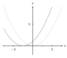
$clipboard_e13b260cf71178c6038e3db08e9c5f34a.png$

Figure $\PageIndex{18}$: Quadratic Shift

then, we shrink the function horizontally (solid):

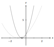
$clipboard_e80fea6ece407d048952fdeb1fc75460d.png$

Figure $\PageIndex{19}$: Quadratic shift shrink

Notice that when we shrink it, the point on the y-axis, $(0,1)$, is the only point that is the same between both graphs. This is because we shrink and stretch around the y-axis, not around the center of the graph. We can see this also by seeing that the x-intercept changes from $(-1,0)$ to $(-\frac{1}{2},0)$ (labeled with an open dot).

If a function is being modified both vertically and horizontally, you should take care of all the horizontal changes first. Let’s see how this looks.

Example $\PageIndex{6}$: Graph Transformation

Graph the function $g(x)=-(\frac{1}{2}x+2)^2+3$.

Solution

As with our previous examples, the first step is to identify the base function. Here our base functions is $x^2$ (dotted). We said that we should start with horizontal changes, so let’s look at those first. With horizontal modifications, we need to work with the shift and then the stretch. Inside of our function we have $+2$; this tells us we start by shifting left 2 units (solid):

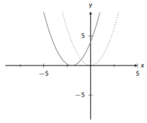
$clipboard_e13b81eec363e33a5b31338ff02bba811.png$

Figure $\PageIndex{20}$: Quadratic Transformation

Next, we will stretch our graph horizontally (solid) by a factor of 2 since $x$ is multiplied by $\frac{1}{2}$ on the inside of the function:

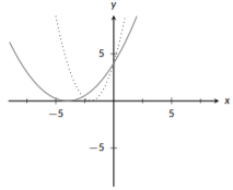
$clipboard_e7f8e478d1c70d1f55e3cd9ff6d06b0d0.png$

Figure $\PageIndex{21}$: Quadratic Transformation

Now that we have completed all horizontal changes, we can work on vertical changes. We have two: a flip and a shift. We need to do the flip first (solid):

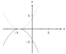
$clipboard_ebc8a8003b191b7144d36faf284bb485b.png$

Figure $\PageIndex{22}$: Quadratic Transformation

The last modification to complete is a shift up 3 units (solid):

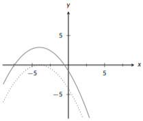
$clipboard_ec4350d71702ab51f27b92ef3245644a0.png$

Figure $\PageIndex{23}$: Quadratic Transformation

In all of our examples so far, we’ve been given the transformed function and asked to graph it. What if we are asked to come up with the new function?

Example $\PageIndex{7}$: Functions for a Transformation

Determine the equation for the graph of $f(x)=x^3$ after it has been shifted 2 units to the right, flipped vertically, and shifted 2 units up.

Solution

Here the transformations have been given in the same order that we would apply them. Our first step, is to shift the function to the right, so we will change to $(x-2)^3$. Next, we want to flip the function vertically, so we get $-(x-2)^3$. Finally, we want to shift up 2 units, so we get $g(x)=-(x-2)^3+2$ as our new function. we gave the function a new name $g$, instead of $f$ so that we won’t get confused by using the same name for both.

2.4.3: Graphs of Piecewise Functions

The last graphing topic we will discuss in this section is graphing piecewise functions. A piecewise function is a function that is defined in pieces; for part of its domain it is defined one way and for other parts it is defined differently. When graphing these functions, the trickiest part is making sure you use the correct piece of the function definition for each part of the domain. To make this a little easier to keep straight, we make sure to only graph one piece at a time.

When switching between different pieces, it is important to do so properly. Sometimes the “end” point of that piece is not actually included. This happens when the domain for that piece is open, i.e., it doesn’t include that final point. This is indicated by a parenthesis or a “$<$” or a “$>$” telling us that the end point should not be included. Here, we would plot an open dot, a circle with a white interior, to show that it is not included. If the endpoint is included, we will plot a closed dot, a circle with a filled in interior, to show that it is included. If the function’s domain for a piece continues all the way to $\infty$ or to $-\infty$, we will indicate this by drawing a small arrow tip at the edge of the graph to show that it continues forever.

Example $\PageIndex{8}$: Graphing a Piecewise Function

Graph the function $f(x) = \left\{\begin{array}{cc} 3-x & 0<x \leq 1 \\ x^2 & 1<x<2 \end{array}\right.$

Solution

This function has two pieces: a line when $x$ is in $(0,1]$ and a quadratic function when $x$ is in $(1,2)$. We like to work from left to right, so we will graph the line first, but you could graph the pieces in any order.

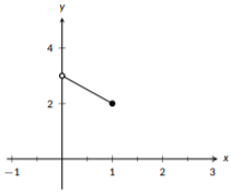
$clipboard_e618d8b71d8b096c1cf73ff62adec5583.png$

Figure $\PageIndex{24}$: Piecewise

Here, we graphed the line by plotting the two end points and connecting them. Since they are the endpoints, we don’t want to move past them. Since the line applied when $0<x\leq1$, we plotted an open dot for $x=0$ to show that it is not included and a closed dot for $x=1$ to show that it is included.

Next, we’ll add the quadratic piece to this graph.

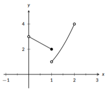
$clipboard_ef2d958eb08727726079aabd53cee12fc.png$

Figure $\PageIndex{25}$: Piecewise

With the quadratic, both ends are open since this piece only applies when $1<x<2$. This means we need open dots at both ends.