4.1: Graphing with the TI-84

Last updated
Save as PDF

Page ID: 48968

Thomas Tradler and Holly Carley
CUNY New York City College of Technology via New York City College of Technology at CUNY Academic Works

$ \newcommand{\vecs}[1]{\overset { \scriptstyle \rightharpoonup} {\mathbf{#1}} } $ $ \newcommand{\vecd}[1]{\overset{-\!-\!\rightharpoonup}{\vphantom{a}\smash {#1}}} $$\newcommand{\id}{\mathrm{id}}$ $ \newcommand{\Span}{\mathrm{span}}$ $ \newcommand{\kernel}{\mathrm{null}\,}$ $ \newcommand{\range}{\mathrm{range}\,}$ $ \newcommand{\RealPart}{\mathrm{Re}}$ $ \newcommand{\ImaginaryPart}{\mathrm{Im}}$ $ \newcommand{\Argument}{\mathrm{Arg}}$ $ \newcommand{\norm}[1]{\| #1 \|}$ $ \newcommand{\inner}[2]{\langle #1, #2 \rangle}$ $ \newcommand{\Span}{\mathrm{span}}$ $\newcommand{\id}{\mathrm{id}}$ $ \newcommand{\Span}{\mathrm{span}}$ $ \newcommand{\kernel}{\mathrm{null}\,}$ $ \newcommand{\range}{\mathrm{range}\,}$ $ \newcommand{\RealPart}{\mathrm{Re}}$ $ \newcommand{\ImaginaryPart}{\mathrm{Im}}$ $ \newcommand{\Argument}{\mathrm{Arg}}$ $ \newcommand{\norm}[1]{\| #1 \|}$ $ \newcommand{\inner}[2]{\langle #1, #2 \rangle}$ $ \newcommand{\Span}{\mathrm{span}}$$\newcommand{\AA}{\unicode[.8,0]{x212B}}$

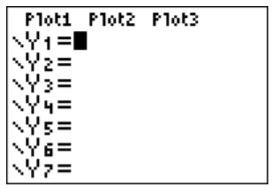
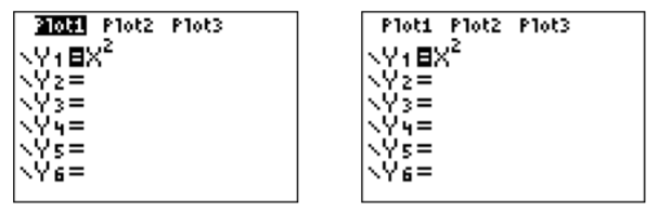
We now use the TI-84 to graph functions such as the functions discussed in the previous chapters. We start by graphing the very well-known function $y=x^2$, which is of course a parabola. To graph $y=x^2$, we first have to enter the function. Press the $\boxed {y =}$ key to get to the function menu:

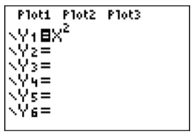
$clipboard_e5be603eec9419d658fa0c0fd3bcd675c.png$

In the first line, enter the function $y=x^2$ by pressing the buttons $\boxed {X,T,\theta ,n} $ for the variable “$x$,” and then press the button $\boxed {x^2}$. We obtain

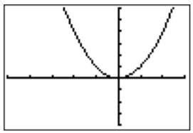
$clipboard_e8af10abcc986f8cbcbf36650317f21a1.png$

We now go to the graphing window by pressing the $\boxed {\text{graph}}$ key. We obtain:

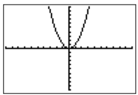
$clipboard_ee9cf040a777d6a4f061a036b8fbb6583.png$

Here, the viewing window is displayed in its initial and standard setting between $-10$ and $10$ on the $x$-axis, and between $-10$ and $10$ on the $y$-axis. These settings may be changed by pressing the $\boxed {\text{window}}$ or the $\boxed {\text{zoom}}$ keys. First, pressing $\boxed {\text{window}}$, we may change the scale by setting Xmin, Xmax, Ymin and Ymax to some new values using $\boxed {\bigtriangledown }$ and $\boxed {\text{enter}}$:

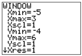
$clipboard_ef50b99eb8f49f68883a1ad1ac8f012d5.png$

Note, that negative numbers have to be entered via $\boxed {(-)}$ and not using $\boxed {-}$.

Note

The difference between $\boxed {(-)}$ and $\boxed {-}$ is that $\boxed {(-)}$ is used to denote negative numbers (such as $-10$), whereas $\boxed {-}$ is used to subtract two numbers (such as $7-3$).

Note

A source for a common error occurs when the “Plot1" item in the function menu is highlighted. When graphing a function as above, always make sure that none of the “plots” are highlighted.

$clipboard_e4a626668020b272ccdc144c3494877a8.png$

After changing the minimum and maximum $x$- and $y$-values of our window, we can see the result after pressing $\boxed {\text{graph}}$ again:

$clipboard_eed1c026ca4f59528108fa5cd1f637cbb.png$

We may zoom in or out or put the setting back to the standard viewing size by pressing the $\boxed {\text{zoom}}$ key:

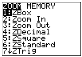
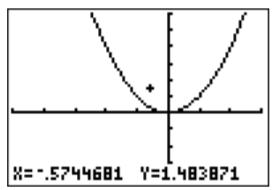
$clipboard_eaa795f9e3b0b779ac333e9cde7913f7e.png$

We may zoom in by pressing $\boxed {2}$, then choose a center in the graph where we want to focus (via the$\boxed {\bigtriangleup }$, $\boxed {\bigtriangledown }$, $\boxed {\triangleleft }$, $\boxed {\triangleright }$ keys), and confirm this with $\boxed {\text{enter}}$:

$clipboard_eb38076933b1a3d9a870e25dab8e0f869.png$

Similarly, we may also zoom out (pressing using $\boxed {3}$ in the zoom menu and choosing a center). Finally we can recover the original setting by using ZStandard in the zoom menu (press $\boxed {6}$).

We can graph more than one function in the same window, which we show next.

Example $\PageIndex{1}$

Graph the equations $y=\sqrt{7-x}$ and $y=x^3-2x^2-4$ in the same window.

Solution

Enter the functions as Y1 and Y2 after pressing $\boxed {y=}$.

The graphs of both functions appear together in the graphing window:

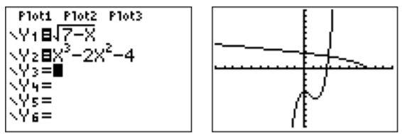
$clipboard_e198d5a8a3347c4431b64e958ab4e0626.png$

Here, the square root symbol “$\sqrt{\,\,}$” is obtained using $\boxed {2\text{nd}}$ and $\boxed {x^2}$, and the third power via $\boxed {\wedge}$ and $\boxed {3}$ (followed by $\boxed {\triangleright }$ to continue entering the function on the base line).

Example $\PageIndex{2}$

Graph the relation $(x-3)^2+(y-5)^2=16$.

Solution

Since the above expression is not solved for $y$, we cannot simply plug this into the calculator. Instead, we have to solve for $y$ first.

\[\begin{aligned} (x-3)^2+(y-5)^2=16 &\implies & (y-5)^2=16-(x-3)^2 \\ &\implies & y-5=\pm \sqrt{16-(x-3)^2} \\ &\implies & y=5\pm \sqrt{16-(x-3)^2} \end{aligned} \nonumber \]

Note, that there are two functions that we need to graph: $y=5+\sqrt{16-(x-3)^2}$ and $y=5-\sqrt{16-(x-3)^2}$. Entering these as Y1 and Y2 in the calculator gives the following function menu and graphing window:

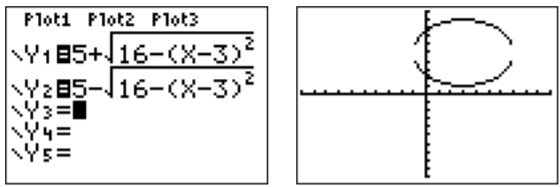
$clipboard_e8eecbdc6836332335b0cc063f660d666.png$

The graph displays a circle of radius $4$ with a center at $(3,5)$. However, due to the current scaling, the graph looks more like an ellipse instead of a circle. We can remedy this by using the “zoom square” function; press $\boxed {\text{zoom}}$ $\boxed {5}$. This adjusts the axis to the same scale in the $x$- and the $y$-direction. We obtain the following graph:

$clipboard_ec76c761cbecc67ee36f4b69e3ac4541d.png$

Note

We recall that the equation $(x-h)^2+(y-k)^2=r^2$ always forms a circle in the plane. Indeed, this equation describes a circle with center $C(h,k)$ and radius $r$.

Note

Note

Example \(\PageIndex{1}\)

Example \(\PageIndex{2}\)

Note