26.4: A.4- Graphing a piecewise defined function

Last updated
Save as PDF

Page ID: 54491

Thomas Tradler and Holly Carley
CUNY New York City College of Technology via New York City College of Technology at CUNY Academic Works

$ \newcommand{\vecs}[1]{\overset { \scriptstyle \rightharpoonup} {\mathbf{#1}} } $ $ \newcommand{\vecd}[1]{\overset{-\!-\!\rightharpoonup}{\vphantom{a}\smash {#1}}} $$\newcommand{\id}{\mathrm{id}}$ $ \newcommand{\Span}{\mathrm{span}}$ $ \newcommand{\kernel}{\mathrm{null}\,}$ $ \newcommand{\range}{\mathrm{range}\,}$ $ \newcommand{\RealPart}{\mathrm{Re}}$ $ \newcommand{\ImaginaryPart}{\mathrm{Im}}$ $ \newcommand{\Argument}{\mathrm{Arg}}$ $ \newcommand{\norm}[1]{\| #1 \|}$ $ \newcommand{\inner}[2]{\langle #1, #2 \rangle}$ $ \newcommand{\Span}{\mathrm{span}}$ $\newcommand{\id}{\mathrm{id}}$ $ \newcommand{\Span}{\mathrm{span}}$ $ \newcommand{\kernel}{\mathrm{null}\,}$ $ \newcommand{\range}{\mathrm{range}\,}$ $ \newcommand{\RealPart}{\mathrm{Re}}$ $ \newcommand{\ImaginaryPart}{\mathrm{Im}}$ $ \newcommand{\Argument}{\mathrm{Arg}}$ $ \newcommand{\norm}[1]{\| #1 \|}$ $ \newcommand{\inner}[2]{\langle #1, #2 \rangle}$ $ \newcommand{\Span}{\mathrm{span}}$$\newcommand{\AA}{\unicode[.8,0]{x212B}}$

Suppose you wanted to graph the piecewise defined function

\[f(x)= \begin{cases}x^{2}, & x<2 \\ 2 x-7, & x \geq 2\end{cases} \nonumber \]

Go to the menu. We need to enter the function in the following way:

\[y=x^2(x<2)+(2x-7)(x\geq 2) \nonumber \]

The only new entries are in the inequality signs, which can be accessed through the “TEST” menu ($\boxed{\text{2nd}}$$\boxed{\text{math}}$).

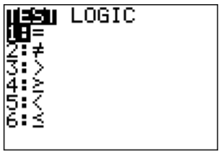
$clipboard_e00458173c770b3ce1d25c933f8a92b83.png$

Therefore, we press the keys: $\boxed{\text{X,T,}\theta,n}$$\boxed{x^2}$$\boxed{\text{(}}$$\boxed{\text{X,T,}\theta,n}$$\boxed{\text{2nd}}$$\boxed{\text{math}}$$\boxed{\text{5}}$$\boxed{\text{2}}$$\boxed{\text{)}}$$\boxed{\text{+}}$$\boxed{\text{(}}$$\boxed{\text{2}}$$\boxed{\text{X,T,}\theta,n}$$\boxed{\text{-}}$$\boxed{\text{7}}$$\boxed{\text{)}}$$\boxed{\text{(}}$$\boxed{\text{X,T,}\theta,n}$$\boxed{\text{2nd}}$$\boxed{\text{math}}$$\boxed{\text{4}}$$\boxed{\text{2}}$$\boxed{\text{)}}$$\boxed{\text{enter}}$. The graph is displayed on the right:

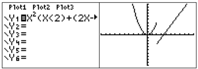
$clipboard_ecdb4a1e4a5c2fcdbbd440e748f853fdc.png$

The meaning of $y=(x<2)$ as a function is that it is equal to $1$ when it is true and $0$ when it is false. In other words, the expression $(x<2)$ is $1$ when $x<2$ and $0$ otherwise. You can use this idea to graph more complicated functions. For example to enter $x+2$ for $0<x<3$ you could enter $(x+2)(0<x)(x<3)$.

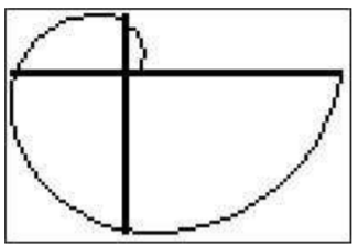
Note: When graphing piecewise defined functions the graph is sometimes different from what is expected. See the common errors section to interpret the resulting graph below.

Graphing with polar coordinates

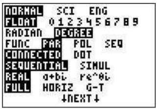
Suppose you want to graph the curve $r=\theta+\sin\theta$. Press $\boxed{\text{mode}}$. On the fourth line highlight ’Pol’ and press $\boxed{\text{enter}}$ (make sure you in radian mode also)

$clipboard_eb6f5b42496732d9ff319110b51c706b2.png$

and press $\boxed{y=}$. Your menu will have a list $r_1, r_2,...$. After $r_1$ type $\boxed{\text{X,T,}\theta,n}$$\boxed{\text{+}}$$\boxed{\sin}$$\boxed{\text{X,T,}\theta,n}$$\boxed{\text{)}}$. Then to see the graph type $\boxed{\text{graph}}$. You may have to adjust your window (zoom fit) to see the resulting spiral.

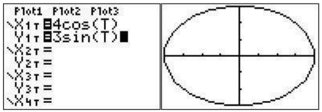
$clipboard_e627ad93867bd053e1e42021e6f9ed5a7.png$

Graphing with parametric coordinates

Suppose you want to graph the curve given by $y(t)=3\sin(t), x(t)=4\cos(t)$. First we need to set the mode to parametric mode: press $\boxed{\text{mode}}$ and highlight ’PAR’ in the fourth line and press $\boxed{\text{enter}}$.

$clipboard_eef3892a9905431d18364c130a7a7af89.png$

Now go to the graphing screen . You will see a list that begins with X$_{1T}$ and Y$_{1T}$. To the right of X$_{1T}$ type $\boxed{\text{4}}$$\boxed{\cos}$$\boxed{\text{X,T,}\theta,n}$ and to the right of Y$_{1T}$ type $\boxed{\text{3}}$$\boxed{\sin}$$\boxed{\text{X,T,}\theta,n}$. Then to see the graph press $\boxed{\text{graph}}$. You may need to $\boxed{\text{zoom}}$$\boxed{\text{0}}$ (zoomfit) to see the resulting ellipse. (Also, be aware that the scale may be misleading– you may want to $\boxed{\text{zoom}}$$\boxed{\text{5}}$ for a clearer understanding of the graph).

$clipboard_e7936156a4fcf3180efef0b83a3b0badc.png$