7.1: Networks and Actors

The social network perspective emphasizes multiple levels of analysis. Differences among actors are traced to the constraints and opportunities that arise from how they are embedded in networks; the structure and behavior of networks grounded in, and enacted by local interactions among actors. As we examine some of the basic concepts and definitions of network analysis in this and the next several chapters, this duality of individual and structure will be highlighted again and again.

In this chapter we will examine some of the most obvious and least complex ideas of formal network analysis methods. Despite the simplicity of the ideas and definitions, there are good theoretical reasons (and some empirical evidence) to believe that these basic properties of social networks have very important consequences. For both individuals and for structures, one main question is connections. Typically, some actors have lots of connections, others have fewer. Some networks are well-connected or "cohesive", others are not. The extent to which individuals are connected to others, and the extent to which the network as a whole is integrated are two sides of the same coin.

Differences among individuals in how connected they are can be extremely consequential for understanding their attributes and behavior. More connections often mean that individuals are exposed to more, and more diverse, information. Highly connected individuals may be more influential, and may be more influenced by others. Differences among whole populations in how connected they are can be quite consequential as well. Disease and rumors spread more quickly where there are high rates of connection. But, so too does useful information. More connected populations may be better able to mobilize their resources, and may be better able to bring multiple and diverse perspectives to bear to solve problems. In between the individual and the whole population, there is another level of analysis - that of "composition". Some populations may be composed of individuals who are all pretty much alike in the extent to which they are connected. Other populations may display sharp differences, with a small elite of central and highly connected persons, and larger masses of persons with fewer connections. Differences in connections can tell us a good bit about the stratification order of social groups. A great deal of recent work by Duncan Watts, Doug White and many others outside of the social sciences is focusing on the consequences of variation in the degree of connection of actors.

Because most individuals are not usually connected directly to most other individuals in a population, it can be quite important to go beyond simply examining the immediate connections of actors, and the overall density of direct connections in populations. The second major (but closely related) set of approaches that we will examine in this chapter have to do with the idea of the distance between actors (or, conversely, how close they are to one another). Some actors may be able to reach most other members of the population with little effort: they tell their friends, who tell their friends, and "everyone" knows. Other actors may have difficulty being heard. They may tell people, but the people they tell are not well connected, and the message doesn't go far. Thinking about it the other way around, if all of my friends have one another as friends, my network is fairly limited - even though I may have quite a few friends. But, if my friends have many non-overlapping connections, the range of my connection is expanded. If individuals differ in their closeness to other actors, then the possibility of stratification along this dimension arises. Indeed, one major difference among "social classes" is not so much in the number of connections that actors have, but in whether these connections overlap and "constrain" or extend outward and provide "opportunity". Populations as a whole, then, can also differ in how close actors are to other actors, on the average. Such differences may help us to understand diffusion, homogeneity, solidarity, and other differences in macro properties of social groups.

Social network methods have a vocabulary for describing connectedness and distance that might, at first, seem rather formal and abstract. This is not surprising, as many of the ideas are taken directly from the mathematical theory of graphs. But it is worth the effort to deal with the jargon. The precision and rigor of the definitions allow us to communicate more clearly about important properties of social structures - and often lead to insights that we would not have had if we used less formal approaches.

An Example: Knoke's Information Exchange

The basic properties of networks are easier to learn and understand by example. Studying an example also shows sociologically meaningful applications of the formalisms. In this chapter, we will look at a single directed binary network that describes the flow of information among 10 formal organizations concerned with social welfare issues in one mid-western U.S. city (Knoke and Burke). Of course, network data come in many forms (undirected, multiple ties, valued ties, etc.) and one example can't capture all of the possibilities. Still, it can be rather surprising how much information can be "squeezed out" of a single binary matrix by using basic graph concepts.

For small networks, it is often useful to examine graphs. Figure 7.1 shows the di-graph (directed graph) for the Knoke information exchange data:

Figure 7.1: Knoke information exchange directed graph

Your trained eye should immediately perceive a number of things in looking at the graph. There is a limited number of actors here (ten, actually), and all of them are "connected". But, clearly not every possible connection is present, and there are "structural holes" (or at least "thin spots" in the fabric). There appear to be some differences among the actors in how connected they are (compare actor number 7, a newspaper, to actor number 6, a welfare rights advocacy organization). If you look closely, you can see that some actors' connections are likely to be reciprocated (that is, if A shares information with B, B also shares information with A); some other actors (e.g. 6 and 10), are more likely to be senders than receivers of information. As a result of the variation in how connected individuals are, and whether the ties are reciprocated, some actors may be at quite some "distance" from other actors. There appear to be groups of actors who differ in this regard (2, 5, and 7 seem to be in the center of the action; 6, 9, and 10 seem to be more peripheral).

A careful look at the graph can be very useful in getting an intuitive grasp of the important features of a social network. With larger populations or more connections, however, graphs may not be much help. Looking at a graph can give a good intuitive sense of what is going on, but our descriptions of what we see are rather imprecise (the previous paragraph is an example of this). To get more precise, and to use computers to apply algorithms to calculate mathematical measures of graph properties, it is necessary to work with the adjacency matrix instead of the graph. The Knoke data graphed above are shown as an asymmetric adjacency matrix in Figure 7.2.

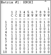
Figure 7.2: Knoke information exchange adjacency matrix

Using Data>Display, we can look at the network in matrix form. There are ten rows and columns, the data are binary, and the matrix is asymmetric. As we mentioned in the chapter on using matrices to represent networks, the row is treated as the source of information and the columns as the receiver. By doing some very simple operations on this matrix it is possible to develop systematic and useful index numbers, or measures, of some of the network properties that our eye discerns in the graph.