4.3: Simulating Discrete-Time Models with One Variable

Now is the time to do our very first exercise of computer simulation of discrete-time models in Python. Let’s begin with this very simple linear difference equation model of a scalar variable \(x\):

\[x_{t}=ax_{t-1}\label{(4.12)} \]

Here, \(a\) is a model parameter that specifies the ratio between the current state and the next state. Our objective is to find out what kind of behavior this model will show through computer simulation.

When you want to conduct a computer simulation of any sort, there are at least three essential things you will need to program, as follows:

Three essential components of computer simulation

Initialize. You will need to set up the initial values for all the state variables of the system.
Observe. You will need to define how you are going to monitor the state of the system. This could be done by just printing out some variables, collecting measurements in a list structure, or visualizing the state of the system.
Update. You will need to define how you are going to update the values of those state variables in every time step. This part will be defined as a function, and it will be executed repeatedly.

We will keep using this three-part architecture of simulation codes throughout this textbook. All the sample codes are available from the textbook’s website at http://bingweb.binghamton.edu/~sayama/textbook/, directly linked from each Code example if you are reading this electronically.

To write the initialization part, you will need to decide how you are going to represent the system’s state in your computer code. This will become a challenging task when we work on simulations of more complex systems, but at this point, this is fairly easy. Since we have just one variable, we can decide to use a symbol \(x\) to represent the state of the system. So here is a sample code for initialization:

In this example, we defined the initialization as a Python function that initializes the global variable \(x\) from inside the function itself. This is why we need to declare that \(x\) is global at the beginning. While such use of global variables is not welcomed in mainstream computer science and software engineering, I have found that it actually makes simulation codes much easier to understand and write for the majority of people who don’t have much experience in computer programming. Therefore,we frequently use global variables throughout this textbook.

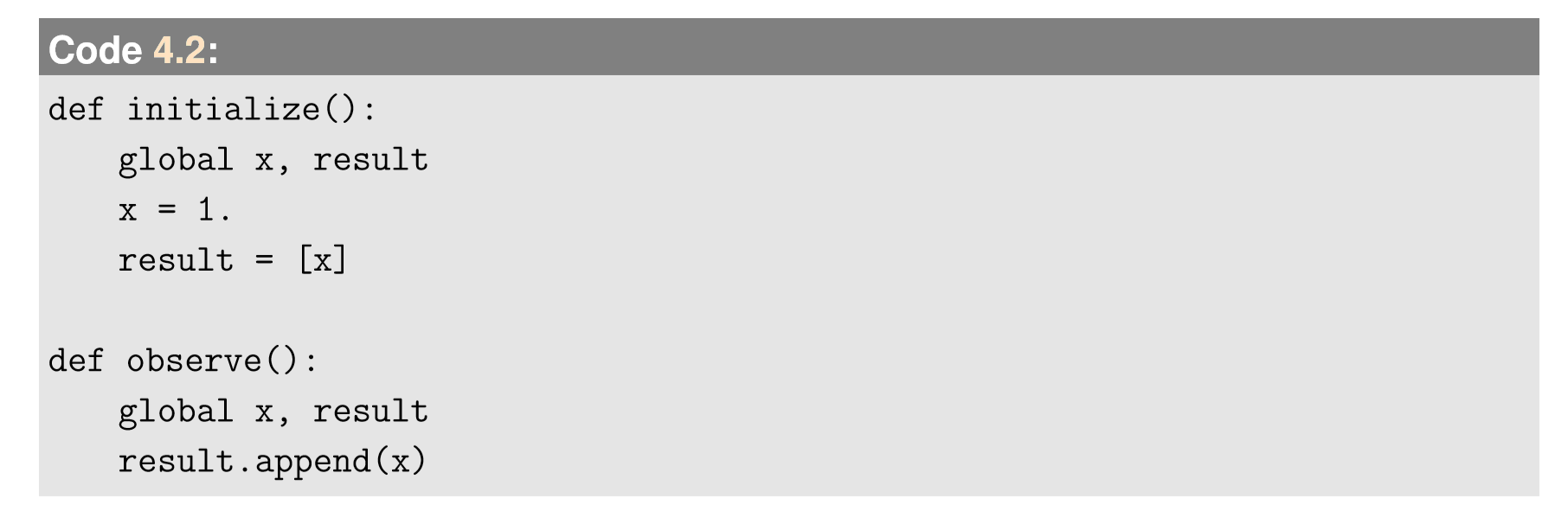
Next, we need to code the observation part. There are many different ways to keep track of the state variables in a computer simulation, but here let’s use a very simple approach to create a time series list. This can be done by first initializing the list with the initial state of the system, and then appending the current state to the list each time the observation is made. We can define the observation part as a function to make it easier to read. Here is the updated code:

Finally, we need to program the updating part. This is where the actual simulation occurs. This can be implemented in another function:

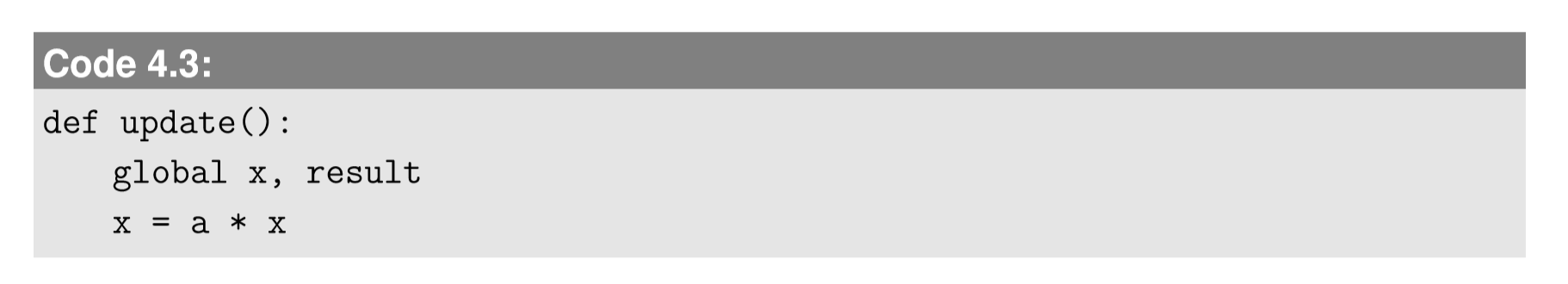
Note that the last line directly overwrites the content of symbol \(x\). There is no distinction between \(x_{t−1}\) and \(x_{t}\),but this is okay, because the past values of \(x\) are stored in the results list in the observe function. Now we have all the three crucial components implemented. We also need to add parameter settings to the beginning, and the iterative loop of updating at the end. Here, let’s let \(a = 1.1\) so that the value of \(x\) increases by 10% in each time step. The completed simulation code looks like this:

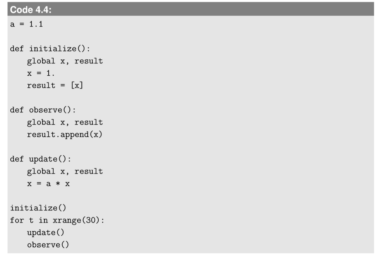
Here we simulate the behavior of the system for 30 time steps. Try running this code inyour Python and make sure you don’t get any errors. If so, congratulations! You have just completed the first computer simulation of a dynamical system. Of course, this code doesn’t produce any output, so you can’t be sure if the simulation ran correctly or not. An easy way to see the result is to add the following line to the end of the code:

If you run the code again, you will probably see something like this:

We see that the value of x certainly grew. But just staring at those numbers won’t give us much information about how it grew. We should visualize these numbers to observe the growth process in a more intuitive manner. To create a visual plot, we will need to use the matplotlib library¹. Here we use its pylab environment included in matplotlib. Pylab provides a MATLAB-like working environment by bundling matplotlib’s plotting functions together with a number of frequently used mathematical/computational functions (e.g., trigonometric functions, random number generators, etc.). To use pylab, you can add the following line to the beginning of your code²:

And then you can add the following lines to the end of your code:

The completed code as a whole is as follows (you can download the actual Python code by clicking on the name of the code in this textbook):

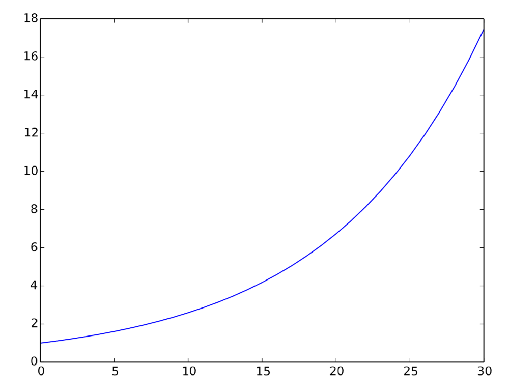
Run this code and you should get a new window that looks like Fig. 4.3.1. If not, check your code carefully and correct any mistakes. Once you get a successfully visualized plot, you can clearly see an exponential growth process in it. Indeed, Equation \ref{(4.12)} is a typical mathematical model of exponential growth or exponential decay. You can obtain several distinct behaviors by varying the value of \(a\).

Figure \(\PageIndex{1}\): Visual output of Code 4.9.

Exercise \(\PageIndex{1}\)

Conduct simulations of this model for various values of parameter a to see what kind of behaviors are possible in this model and how the value of a determines the resulting behavior.

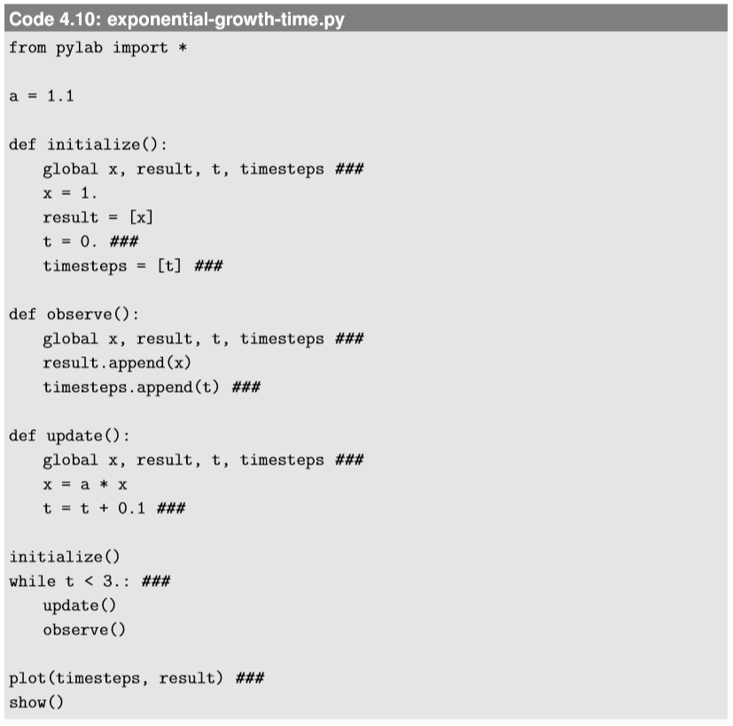
For your information, there are a number of options you can specify in the plot function, such as adding a title, labeling axes, changing color, changing plot ranges, etc. Also, you can manipulate the result of the plotting interactively by using the icons located at the bottom of the plot window. Check out matplotlib’s website (http://matplotlib.org/) to learn more about those additional features yourself. In the visualization above, the horizontal axis is automatically filled in by integers starting with 0. But if you want to give your own time values (e.g., at intervals of 0.1), you can simulate the progress of time as well, as follows (revised parts are marked with ###):

Exercise \(\PageIndex{2}\)

Implement a simulation code of the following difference equation:

\[x_{t} = ax_{t-1} +b, x_{0}=1\label{(4.13)} \]

This equation is still linear, but now it has a constant term in addition to \(ax_{t−1}\). Some real-world examples that can be modeled in this equation include fish population growth with constant removals due to fishing, and growth of credit card balances with constant monthly payments (both with negative \(b\)). Change the values of \(a\) and \(b\), and see if the system’s behaviors are the same as those of the simple exponential growth/decay model

¹It is already included in Anaconda and Enthought Canopy. If you are using a different distribution of Python, matplotlib is freely available from http://matplotlib.org/.

²Another way to import pylab is to write “import pylab” instead, which is recommended by more programming-savvy people. If you do this, however, pylab’s functions have to have the prefix pylab added to them, such as pylab.plot(result). For simplicity, we use “from pylab import *” throughout this textbook