
9.1: Chaos in Discrete-Time Models
- Page ID
- 7817

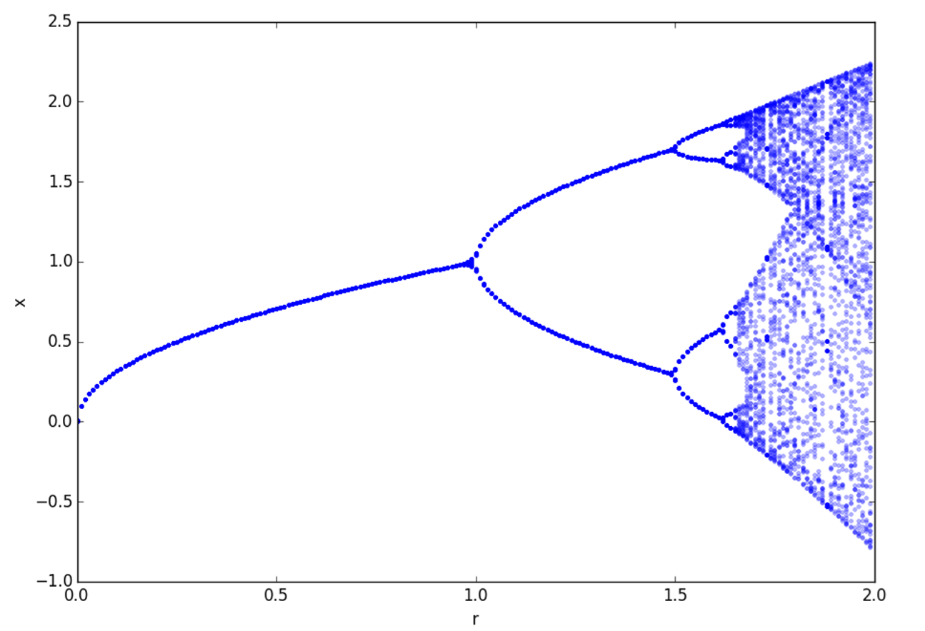
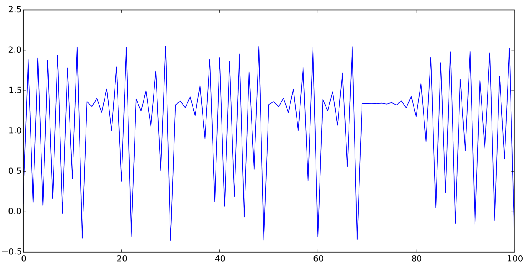
Figure 8.4.3 showed a cascade of period-doubling bifurcations, with the intervals between consecutive bifurcation thresholds getting shorter and shorter geometrically as r increased. This cascade of period doubling eventually leads to the divergence of the period to infinity at \(r ≈ 1.7\) in this case,which indicates the onset of chaos. In this mysterious parameter regime,the system loses any finite-length periodicity, and its behavior looks essentially random. Figure 9.1.1 shows an example of such chaotic behavior of Eq.(8.4.3) with \(r = 1.8\).
So what is chaos anyway? It can be described in a number of different ways, as follows:
- Chaos is a long-term behavior of a nonlinear dynamical system that never falls in any static or periodic trajectories.
- Chaos looks like a random fluctuation, but still occurs in completely deterministic, simple dynamical systems.
- Chaos exhibits sensitivity to initial conditions.
- Chaos occurs when the period of the trajectory of the system’s state diverges to infinity.
- Chaos occurs when no periodic trajectories are stable.
- Chaos is a prevalent phenomenon that can be found everywhere in nature, as well as in social and engineered environments.
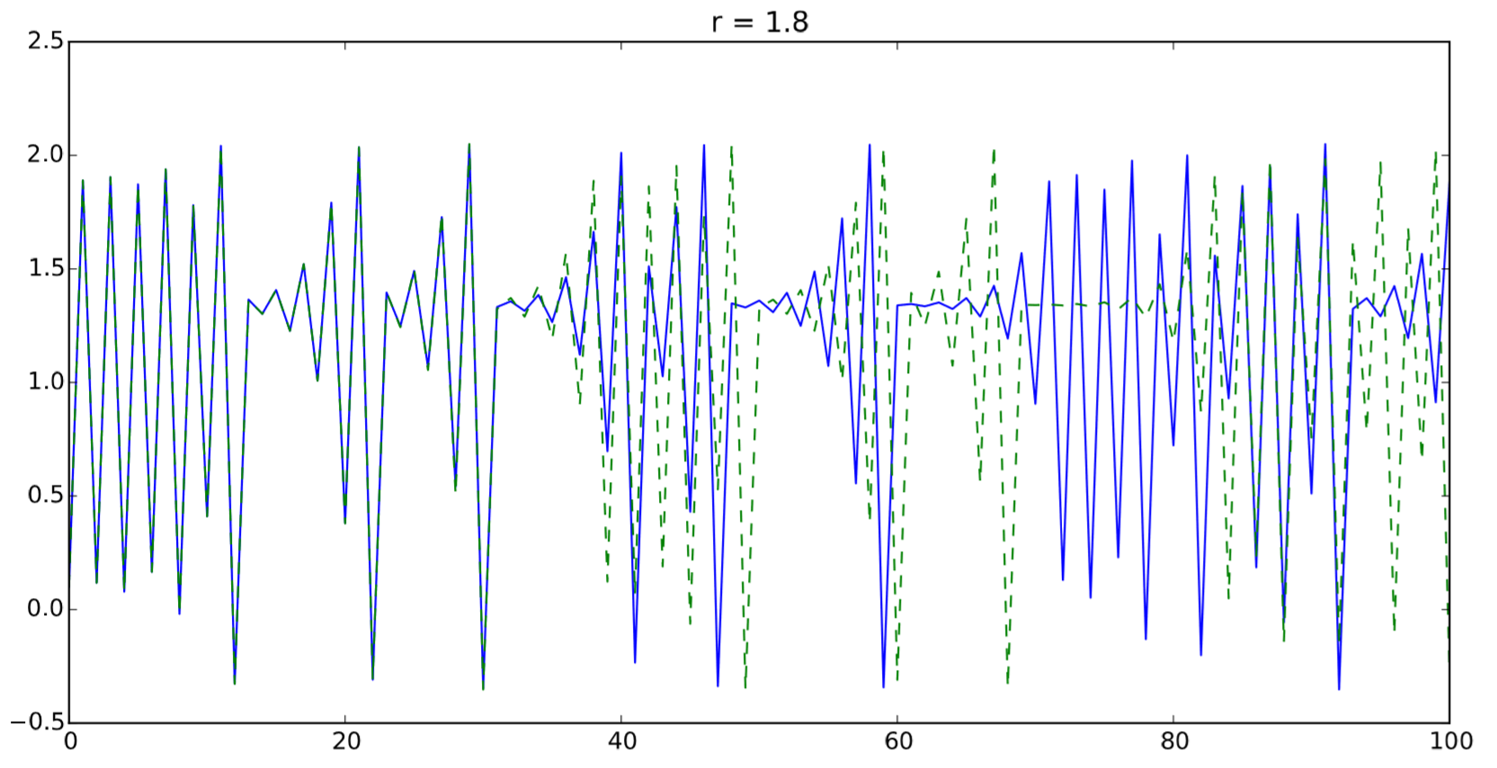
The sensitivity of chaotic systems to initial conditions is particularly well known under the moniker of the “butterfly effect,” which is a metaphorical illustration of the chaotic nature of the weather system in which “a flap of a butterfly’s wings in Brazil could set off a tornado in Texas.” The meaning of this expression is that, in a chaotic system, a small perturbation could eventually cause very large-scale difference in the long run. Figure 9.1.2 shows two simulation runs of Eq. (8.4.3) with \(r = 1.8\) and two slightly different initial conditions, \(x_0 = 0.1\) and \(x_0 = 0.100001\). The two simulations are fairly similar for the first several steps, because the system is fully deterministic (this is why weather forecasts for just a few days work pretty well). But the “flap of the butterfly’s wings” (the 0.000001 difference) grows eventually so big that it separates the long-term fates of the two simulation runs. Such extreme sensitivity of chaotic systems makes it practically impossible for us to predict exactly their long-term behaviors (this is why there are no two-month weather forecasts1).
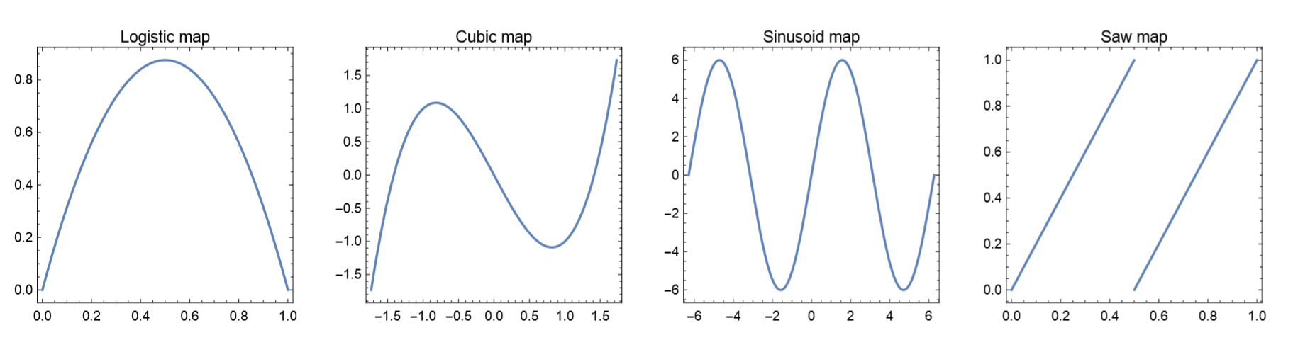
There are many simple mathematical models that exhibit chaotic behavior. Try simulating each of the following dynamical systems (shown in Fig. 9.1.3). If needed, explore and find the parameter values with which the system shows chaotic behaviors.
- Logistic map: \(x_t = rx_{t−1}(1−x_{t−1})\)
- Cubic map: \(x_t = x^{3}_{ t−1} −rx_{t−1}\)
- Sinusoid map: \(x_t = rsinx_{t−1}\)
- Saw map: \(x_t =\) fractional part of \(2x_{t−1}\)
Note: The saw map may not show chaos if simulated on a computer,but it will show chaos if it is manually simulated on a cobweb plot. This issue will be discussed later.
1But this doesn’t necessarily mean we can’t predict climate change over longer time scales. What is not possible with a chaotic system is the prediction of the exact long-term behavior, e.g., when, where, and how much it will rain over the next 12 months. It is possible, though, to model and predict long-term changes of a system’s statistical properties, e.g., the average temperature of the global climate, because it can be described well in a much simpler, non-chaotic model. We shouldn’t use chaos as an excuse to avoid making predictions for our future!