Section Exercises
Verbal
1. Explain the difference between the coefficient of a power function and its degree.
Answer: The coefficient of the power function is the real number that is multiplied by the variable raised to a power. The degree is the highest power appearing in the function.
2. If a polynomial function is in factored form, what would be a good first step in order to determine the degree of the function?
3. In general, explain the end behavior of a power function with odd degree if the leading coefficient is positive.
Answer: As \(x\) decreases without bound, so does \(f(x)\). As \(x\) increases without bound, so does \(f(x)\).
4. What is the relationship between the degree of a polynomial function and the maximum number of turning points in its graph?
5. What can we conclude if, in general, the graph of a polynomial function exhibits the following end behavior? As x→−∞, \(f(x)→−∞\) and as x→∞, \(f(x)→−∞\).
Answer: The polynomial function is of even degree and leading coefficient is negative.
Algebraic
For the following exercises, identify the function as a power function, a polynomial function, or neither.
6. \(f(x)=x^5\)
7. \(f(x)=(x^2)^3\)
Answer: Power function
8. \(f(x)=x−x^4\)
Exercise \(\PageIndex{9}\)
\(f(x)=\frac{x^2}{x^2−1}\)
- Answer
-
Neither
10. \(f(x)=2x(x+2)(x−1)^2\)
11. \(f(x)=3^{x+1}\)
Answer: Neither
For the following exercises, find the degree and leading coefficient for the given polynomial.
12. \(−3x^4\)
13. \(7−2x^2\)
Answer: Degree = 2, Coefficient = –2
14. \(−2x^2− 3x^5+ x−6\)
15. \(x(4−x^2)(2x+1)\)
Answer: Degree =4, Coefficient = –2
16. \(x^2(2x−3)^2\)
For the following exercises, determine the end behavior of the functions.
17. \(f(x)=x^4\)
Answer: As \(x→∞\), \(f(x)→∞\), as \(x→−∞\), \(f(x)→∞\)
18. \(f(x)=x^3\)
19. \(f(x)=−x^4\)
Answer: As \(x→−∞\), \(f(x)→−∞\), as \(x→∞\), \(f(x)→−∞\)
20. \(f(x)=−x^9\)
21. \(f(x)=−2x^4− 3x^2+ x−1\)
Answer: As \(x→−∞\), \(f(x)→−∞\), as \(x→∞\), \(f(x)→−∞\)
22. \(f(x)=3x^2+ x−2\)
23. \(f(x)=x^2(2x^3−x+1)\)
Answer: As \(x→∞\), \(f(x)→∞\), as \(x→−∞\), \(f(x)→−∞\)
24. \(f(x)=(2−x)^7\)
For the following exercises, find the intercepts of the functions.
25. \(f(t)=2(t−1)(t+2)(t−3)\)
Answer: y-intercept is \((0,12)\), t-intercepts are \((1,0);(–2,0); \) and \((3,0)\).
26. \(g(n)=−2(3n−1)(2n+1)\)
Exercise \(\PageIndex{27}\)
\(f(x)=x^4−16\)
- Answer
-
y-intercept is \((0,−16).\) x-intercepts are \((2,0)\) and \((−2,0)\).
28. \(f(x)=x^3+27\)
29. \(f(x)=x(x^2−2x−8)\)
Answer: y-intercept is \((0,0)\). x-intercepts are \((0,0),(4,0),\) and \((−2, 0)\).
30. \(f(x)=(x+3)(4x^2−1)\)
Graphical
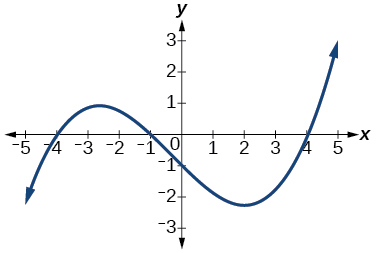
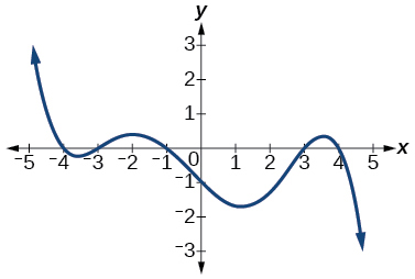
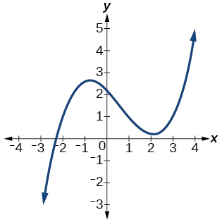
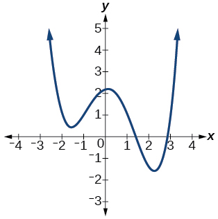
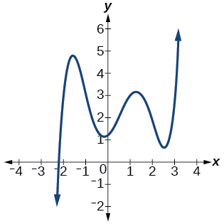
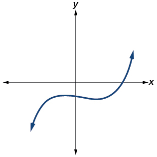
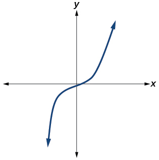
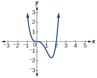
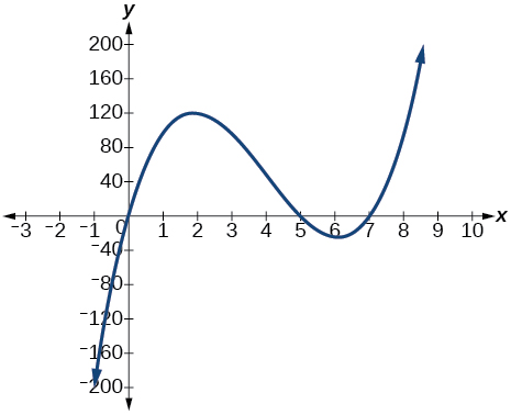
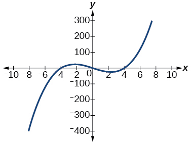
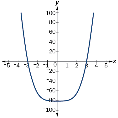
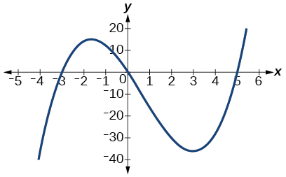
For the following exercises, determine the least possible degree of the polynomial function shown.
31.

Answer: 3
32.

33.

Answer: 5
34.

35.

Answer: 3
36.

37.

Answer: 5
38.

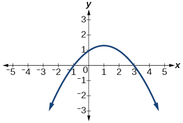
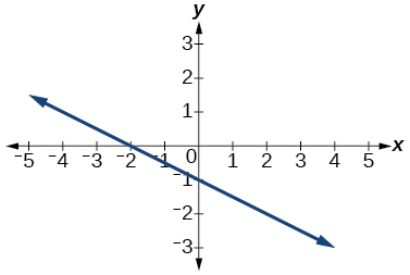
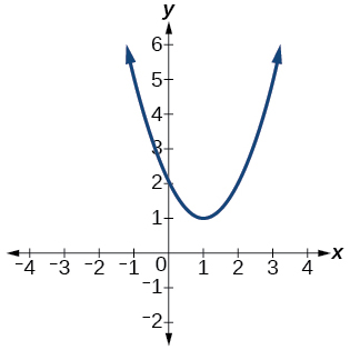
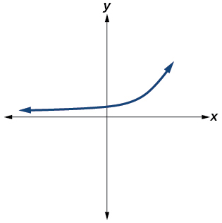
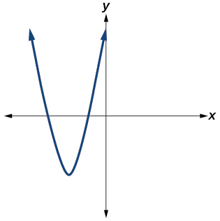
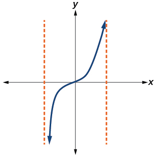
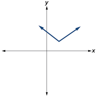
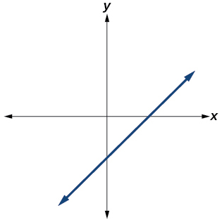
For the following exercises, determine whether the graph of the function provided is a graph of a polynomial function. If so, determine the number of turning points and the least possible degree for the function.
39.

Answer: Yes. Number of turning points is 2. Least possible degree is 3.
40.

41.

Answer: Yes. Number of turning points is 1. Least possible degree is 2.
42.

43.

Answer: Yes. Number of turning points is 0. Least possible degree is 3.
Exercise \(\PageIndex{44}\)

- Answer
-
No (the graph is not smooth)
45.

Answer: Yes. Number of turning points is 0. Least possible degree is 1.
Numeric
For the following exercises, make a table to confirm the end behavior of the function.
46. \(f(x)=−x^3\)
47. \(f(x)=x^4−5x^2\)
Answer:
| \(x\) |
\(f(x)\) |
| 10 |
9,500 |
| 100 |
99,950,000 |
| –10 |
9,500 |
| –100 |
99,950,000 |
as \(x→−∞,\) \(f(x)→∞\), as \(x→∞,\) \(f(x)→∞\)
48. \(f(x)=x^2(1−x)^2\)
49. \(f(x)=(x−1)(x−2)(3−x)\)
Answer:
| \(x\) |
\(f(x)\) |
| 10 |
9,500 |
| 100 |
99,950,000 |
| –10 |
9,500 |
| –100 |
99,950,000 |
as \(x→−∞,\) \(f(x)→∞\), as \(x→∞,\) \(f(x)→−∞\)
50. \(f(x)=\frac{x^5}{10}−x^4\)
Technology
For the following exercises, graph the polynomial functions using a calculator. Based on the graph, determine the intercepts and the end behavior.
51. \(f(x)=x^3(x−2)\)
Answer:

The y-intercept is \((0, 0)\). The x-intercepts are \((0, 0), (2, 0).\) As \(x→−∞,\) \(f(x)→∞\), as \(x→∞,\) \(f(x)→∞\)
52. \(f(x)=x(x−3)(x+3)\)
53. \(f(x)=x(14−2x)(10−2x)\)
Answer:

The y-intercept is \((0,0)\) . The x-intercepts are \((0, 0), (5, 0), (7, 0)\). As \(x→−∞\), \(f(x)→−∞\), as \(x→∞,\) \(f(x)→∞\)
54. \(f(x)=x(14−2x)(10−2x)^2\)
55. \(f(x)=x^3−16x\)
Answer:

The y-intercept is (0, 0). The x-intercept is \((−4, 0), (0, 0), (4, 0)\). As \(x→−∞\), \(f(x)→−∞\), as \(x→∞,\) \(f(x)→∞\)
56. \(f(x)=x^3−27\)
57. \(f(x)=x^4−81\)
Answer:

The y-intercept is (0, −81). The x-intercept are \((3, 0), (−3, 0)\). As \(x→−∞,\) \(f(x)→∞\), as \(x→∞,\) \(f(x)→∞\)
58. \(f(x)=−x^3+x^2+2x\)
59. \(f(x)=x^3−2x^2−15x\)
Answer:

The y-intercept is \((0, 0)\). The x-intercepts are \((−3, 0), (0, 0), (5, 0).\) As \(x→−∞\), \(f(x)→−∞\), as \(x→∞,\) \(f(x)→∞\)
60. \(f(x)=x^3−0.01x\)
Extensions
For the following exercises, use the information about the graph of a polynomial function to determine the function. Assume the leading coefficient is 1 or –1. There may be more than one correct answer.
61. The y-intercept is \((0,−4)\). The x-intercepts are \((−2,0), (2,0)\). Degree is 2.
End behavior: as \(x→−∞,\) \(f(x)→∞\), as \(x→∞,\) \(f(x)→∞\).
Answer: \(f(x)=x^2−4\)
62. The y-intercept is \((0,9)\). The x-intercepts are \((−3,0), (3,0)\). Degree is 2.
End behavior: as \(x→−∞,\) \(f(x)→−∞\), as \(x→∞,\) \(f(x)→−∞\).
63. The y-intercept is \((0,0)\). The x-intercepts are \((0,0), (2,0)\). Degree is 3.
End behavior: as \(x→−∞,\) \(f(x)→−∞\), as \(x→∞,\) \(f(x)→∞\).
Answer: \(f(x)=x^3−4x^2+4x\)
64. The y-intercept is \((0,1)\). The x-intercept is \((1,0)\). Degree is 3.
End behavior: as \(x→−∞\), \(f(x)→∞\), as \(x→∞\), \(f(x)→−∞\).
65. The y-intercept is \((0,1)\). There is no x-intercept. Degree is 4.
End behavior: as \(x→−∞,\) \(f(x)→∞\), as \(x→∞,\) \(f(x)→∞\).
Answer: \(f(x)=x^4+1\)
Real-World Applications
For the following exercises, use the written statements to construct a polynomial function that represents the required information.
66. An oil slick is expanding as a circle. The radius of the circle is increasing at the rate of 20 meters per day. Express the area of the circle as a function of \(d\), the number of days elapsed.
67. A cube has an edge of 3 feet. The edge is increasing at the rate of 2 feet per minute. Express the volume of the cube as a function of \(m\), the number of minutes elapsed.
Answer: \(V(m)=8m^3+36m^2+54m+27\)
68. A rectangle has a length of 10 inches and a width of 6 inches. If the length is increased by \(x\) inches and the width increased by twice that amount, express the area of the rectangle as a function of \(x\).
Exercise \(\PageIndex{69}\)
An open box is to be constructed by cutting out square corners of \(x\)-inch sides from a piece of cardboard 8 inches by 8 inches and then folding up the sides. Express the volume of the box as a function of \(x\).
- Answer
-
\(V(x)=4x^3−32x^2+64x\)
70. A rectangle is twice as long as it is wide. Squares of side 2 feet are cut out from each corner. Then the sides are folded up to make an open box. Express the volume of the box as a function of the width (x).


