4.6: Dividing Polynomials

Learning Objectives

• Use long division to divide polynomials.
• Use synthetic division to divide polynomials.

The exterior of the Lincoln Memorial in Washington, D.C., is a large rectangular solid with length 61.5 meters (m), width 40 m, and height 30 m. We can easily find the volume using elementary geometry.

\[\begin{align*} V&=l \; {\cdot} \; w \; {\cdot} \; h \\ &=61.5 \; {\cdot} \; 40 \; {\cdot} \; 30 \\ &=73,800 \end{align*}\]

So the volume is 73,800 cubic meters (\(m^3\)).

Figure \(\PageIndex{1}\): Lincoln Memorial, Washington, D.C. (credit: Ron Cogswell, Flickr)

Suppose we knew the volume, length, and width. We could divide to find the height.

\[\begin{align*} h&=\dfrac{V}{l{\cdot}w} \\[2pt]&=\dfrac{73,800}{61.5{\cdot}40} \\[2pt] &=30 \end{align*}\]

As we can confirm from the dimensions above, the height is 30 m. We can use similar methods to find any of the missing dimensions. We can also use the same method if any or all of the measurements contain variable expressions. For example, suppose the volume of a rectangular solid is given by the polynomial \(3x^4−3x^3−33x^2+54x\). The length of the solid is given by \(3x\); the width is given by \(x−2\).

To find the height of the solid, we can use polynomial division, which is the focus of this section.

Using Long Division to Divide Polynomials

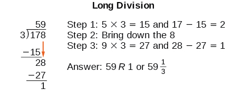
You may recall the long division algorithm for ordinary arithmetic. We begin by dividing into the digits of the dividend that have the greatest place value. We divide, multiply, subtract, include the digit in the next place value position, and repeat. For example, let’s divide 178 by 3 using long division.

To check the answer, we use the following:

\[\begin{align*} \text{dividend}&=(\text{divisor}{\cdot}\text{quotient})+\text{remainder} \\ 178&=(3{\cdot}59)+1 \\ &=177+1 \\ &=178\end{align*}\]

We call this the Division Algorithm and will discuss it more formally after looking at an example.

Division of a polynomial by another polynomial can be done similarly to long division of whole numbers. We can write a polynomial dividend as the product of the divisor and the quotient added to the remainder. The terms of the polynomial division correspond to the digits (and place values) of the whole number division. This method allows us to divide two polynomials. For example, if we were to divide \(2x^3−3x^2+4x+5\) by \(x+2\) using the long division algorithm, it would look like this:

\[ \require{enclose}
\begin{array}{rll}
x+2 \enclose{longdiv}{2x^3 - 3x^2 + 4x + 5}\kern-.2ex && \hbox{Set up the division problem.}\\[4pt]
2x^2 \phantom{00000000}& & \\[-3pt]
x+2 \enclose{longdiv}{2x^3 - 3x^2 + 4x + 5}\kern-.2ex && \hbox{Divide. $2x^3$  divided by  $x$  is  \(2x^2\).}\\[4pt]
2x^2 \phantom{00000000}& & \\[-3pt]
x+2 \enclose{longdiv}{2x^3 - 3x^2 + 4x + 5}\kern-.2ex &&  \\[-3pt]
  \underline{-(2x^3 + 4x^2)\phantom{0000000}} && \hbox{Multiply  $x+2$  by $2x^2$. Subtract.}\\[-3pt]
-7x^2+4x \phantom{000} && \hbox{ Bring down the next term.} \\[4pt]
2x^2 - 7x \phantom{000}& & \\[-3pt]
x+2 \enclose{longdiv}{2x^3 - 3x^2 + 4x + 5}\kern-.4ex && \hbox{Divide. $ -7x^2 $ divided by $ x $ is $ -7x$.}\\[-3pt]
\underline{-(2x^3 + 4x^2)\phantom{0000000}} && \\[-3pt]
-7x^2+4x \phantom{000} && \\[-3pt]
\underline{-(-7x^2 - 14x)\phantom{00}} && \hbox{Multiply $ x+2 $ by $-7x$. Subtract.}\\[-3pt]
18x+5 && \hbox{ Bring down the next term.} \\[4pt]
2x^2 - 7x + 18& & \\[-3pt]
x+2 \enclose{longdiv}{2x^3 - 3x^2 + 4x + 5\phantom{0}}\kern-.2ex && \hbox{Divide. $18x$ divided by $ x $ is $ 18$.}\\[-3pt]
\underline{-(2x^3 + 4x^2)\phantom{0000000}} && \\[-3pt]
-7x^2+4x \phantom{000} && \\[-3pt]
\underline{-(-7x^2 - 14x)\phantom{00}} && \\[-3pt]
18x+5 &&  \\[-3pt]
\underline{-(18x +36)} && \hbox{Multiply $ x+2 $ by $18$. Subtract.}\\[-3pt]
-31
\end{array} \nonumber\] 

We have found

\[\dfrac{2x^3−3x^2+4x+5}{x+2}=2x^2−7x+18−\dfrac{31}{x+2}. \nonumber\]

We can use the Division Algorithm to write

\[2x^3−3x^2+4x+5=(x+2)(2x^2−7x+18)−31, \nonumber\]

which can be used to check our work.  Make sure you can identify the dividend, the divisor, the quotient, and the remainder.

The Division Algorithm

The Division Algorithm states that, given a polynomial dividend \(f(x)\) and a non-zero polynomial divisor \(d(x)\) where the degree of \(d(x)\) is less than or equal to the degree of \(f(x)\), there exist unique polynomials \(q(x)\) and \(r(x)\) such that

\[f(x)=d(x)q(x)+r(x) \nonumber\]

\(q(x)\) is the quotient and \(r(x)\) is the remainder. The remainder is either equal to zero or has degree strictly less than \(d(x)\).

If \(r(x)=0\), then \(d(x)\) divides into \(f(x)\) with no remainder. When this happens, both \(d(x)\) and \(q(x)\) are factors of \(f(x)\).

Given a polynomial \(f(x)\) of degree \(n\) and a polynomial \(d(x)\) of degree less than or equal to \(n\), use long division to divide \(f(x)\) by \(d(x)\)

1. Set up the division problem.
2. Determine the first term of the quotient by dividing the leading term of the dividend by the leading term of the divisor.  Write the answer directly above the like term of the dividend.
3. Multiply the answer by the divisor and write the result below the like terms of the dividend.  Put parentheses around the result.
4. Subtract.  Be sure to distribute the minus sign.
5. Bring down the next term of the dividend.
6. Repeat steps 2–5 until reaching the last term of the dividend.
7. If the remainder is non-zero, express as a fraction using the divisor as the denominator.

Example \(\PageIndex{1}\): Using Long Division to Divide a 2nd-Degree Polynomial by a 1st-degree polynomial

Divide \(5x^2+3x−2\) by \(x+1\).

Solution

\[ \require{enclose}
\begin{array}{rll}
x+1 \enclose{longdiv}{5x^2 + 3x -2}\kern-.2ex && \hbox{Set up the division problem.}\\[4pt]
5x \phantom{000}& & \\[-3pt]
x+1 \enclose{longdiv}{5x^2 + 3x -2}\kern-.2ex && \hbox{Divide. $5x^2$  divided by  $x$  is  \(5x\).}\\[4pt]
5x \phantom{000}& & \\[-3pt]
x+1 \enclose{longdiv}{5x^2 + 3x -2}\kern-.2ex &&  \\[-3pt]
  \underline{-(5x^2 + 5x)\phantom{000}} && \hbox{Multiply  $x+1$  by $5x$. Subtract.}\\[-3pt]
-2x-2  && \hbox{ Bring down the next term.} \\[4pt]
5x-2 & & \\[-3pt]
x+1 \enclose{longdiv}{5x^2 + 3x -2}\kern-.4ex && \hbox{Divide. $ -2x $ divided by $ x $ is $ -2$.}\\[-3pt]
\underline{-(5x^2 + 5x)\phantom{000}} && \\[-3pt]
-2x-2 && \\[-3pt]
\underline{-(-2x-2)}\kern-1ex && \hbox{Multiply $ x+1 $ by $-2$. Subtract.}\\[-3pt]
0
\end{array} \nonumber\]

The quotient is \(5x−2\). The remainder is 0. We write the result as

\[\dfrac{5x^2+3x−2}{x+1}=5x−2 \nonumber\]

or, if we want to use the Division Algorithm to rewrite the polynomial rather than find a quotient,

\[5x^2+3x−2=(x+1)(5x−2) \nonumber\]

Analysis

This division problem had a remainder of 0, which tells us that the divisor and the quotient are factors of the dividend.

Example \(\PageIndex{2}\): Using Long Division to Divide a Third-Degree Polynomial

Divide \(6x^3+11x^2−31x+15\) by \(3x−2\).

Solution

\[ \require{enclose}
\begin{array}{rll}
2x^2  + \; 5x \; - \; 7& & \\[-3pt]
3x-2 \enclose{longdiv}{6x^3 + 11x^2 - 31x + 15}\kern-.2ex && \hbox{$6x^3$ divided by $3x$ is $2x^2$.}\\[-3pt]
\underline{-(6x^3 - \;4x^2)\phantom{000000000}}\kern.2ex && \hbox{Multiply $ 3x-2 $ by $2x^2$. Subtract.}\\[-3pt]
15x^2-31x \phantom{0000}\kern.4ex && \hbox{Bring down the next term. $15x^2$ divided by $3x$ is $5x$.} \\[-3pt]
\underline{-(15x^2 - 10x)\phantom{0000}} && \hbox{Multiply $ 3x-2 $ by $5x$. Subtract.}\\[-3pt]
-21x+15 &&  \hbox{Bring down the next term. $-21x$ divided by $3x$ is $-7$.}\\[-3pt]
\underline{-(-21x +14)}\kern-.4ex && \hbox{Multiply $ 3x-2 $ by $-7$. Subtract.}\\[-3pt]
1 && \hbox{The remainder is 1.}
\end{array} \nonumber\] 

There is a remainder of 1. We can express the result as:

\[\dfrac{6x^3+11x^2−31x+15}{3x−2}=2x^2+5x−7+\dfrac{1}{3x−2} \nonumber\]

Analysis

We can check our work by using the Division Algorithm and simplifying the left-hand side.

\[(3x−2)(2x^2+5x−7)+1=6x^3+11x^2−31x+15 \nonumber\]

Notice, as we write our result,

• the dividend is \(6x^3+11x^2−31x+15\)
• the divisor is \(3x−2\)
• the quotient is \(2x^2+5x−7\)
• the remainder is \(1\)

\(\PageIndex{1}\)

Divide \(16x^3−12x^2+20x−3\) by \(4x+5\).

Solution

\(4x^2−8x+15−\dfrac{78}{4x+5}\)

Using Synthetic Division to Divide Polynomials

As we’ve seen, long division of polynomials can involve many steps and be quite cumbersome. Synthetic division is a shorthand method of dividing polynomials for the special case of dividing by a linear factor whose leading coefficient is 1.

To illustrate the process, recall the example at the beginning of the section.

Divide \(2x^3−3x^2+4x+5\) by \(x+2\) using the long division algorithm.

The final form of the process looked like this:

\[ \require{enclose}
\begin{array}{rll}
2x^2 - 7x + 18& & \\[-3pt]
x+2 \enclose{longdiv}{2x^3 - 3x^2 + 4x + 5\phantom{0}}\kern-.2ex && \\[-3pt]
\underline{-(2x^3 + 4x^2)\phantom{00000000}} && \\[-3pt]
-7x^2+4x \phantom{0000} && \\[-3pt]
\underline{-(-7x^2 - 14x)\phantom{00}} && \\[-3pt]
18x+5 &&  \\[-3pt]
\underline{-(18x +36)}\kern-.3ex && \\[-3pt]
-31
\end{array} \nonumber\] 

There is a lot of repetition in the table. Synthetic division makes the whole process easier to manage. Begin by writing all the coefficients for the dividend, enclosed by a kind of box.  Leave space in the box for more numbers.  On the outside of the box, write the opposite of the constant term in the divisor.  In this example, we write a -2 outside of the box. The process starts by bringing down the leading coefficient, which is 2.

We then multiply the leading coefficient 2 by the -2, write the answer in the next column in the box, and add, repeating this process column by column, until there are no entries left. The bottom row represents the coefficients of the quotient; the last entry of the bottom row is the remainder. In this case, the quotient is \(2x^2–7x+18\) and the remainder is –31.  The process will be made more clear in Example \(\PageIndex{3}\).

Synthetic Division

Synthetic division is a shortcut that can be used when the divisor is a binomial in the form \(x−k\). In synthetic division, only the coefficients of the dividend appear in the division process.

Given two polynomials, use synthetic division to divide

1. Write \(k\) on the outside of the box.
2. Write the coefficients of the dividend inside the box.
3. Bring the lead coefficient down.
4. Multiply the lead coefficient by \(k\). Write the product in the next column.
5. Add the terms of the second column.
6. Multiply the result by \(k\). Write the product in the next column.
7. Repeat steps 5 and 6 for the remaining columns.
8. Use the bottom numbers to write the quotient. The number in the last column is the remainder, the next number from the right has degree 0 (the constant), the next number from the right has degree 1, and so on.  The degree of the quotient is 1 less than the degree of the dividend.

Example \(\PageIndex{3}\): Using Synthetic Division to Divide a Second-Degree Polynomial

Use synthetic division to divide \(5x^2−3x−36\) by \(x−3\).

Solution

Begin by setting up the synthetic division. Write \(k\) and the coefficients.

Bring down the lead coefficient. Multiply the lead coefficient by \(k\), and write the result in the second column.

Add the numbers in the second column. Multiply the resulting number by \(k\).  Write the result in the next column. Then add the numbers in the third column.

The result is \(5x+12\).

The remainder is 0. So \(x−3\) and \(5x+12\) are factors of the original polynomial.

Analysis

Just as with long division, we can check our work by multiplying the quotient by the divisor and adding the remainder.

\[(x−3)(5x+12)+0=5x^2−3x−36 \nonumber\]

Example \(\PageIndex{4}\): Using Synthetic Division to Divide a Third-Degree Polynomial

Use synthetic division to divide \(4x^3+10x^2−6x−20\) by \(x+2\).

Solution

The binomial divisor is \(x+2\) so \(k=−2\). Add each column, multiply the result by –2, and repeat until the last column is reached.

\[{\begin{array}{c}-2\\ \\ \\ \end{array}}{\begin{align*}&\\[0pt]&{\begin{array}{r|}\\[0pt] \\[0pt] \end{array}}\\[1pt]& \\[2pt]& \end{align*}}\!\!
{\begin{array}{rrrr}
4 & 10 & -6 & -20\\
& -8 & -4 & 20 \\
\hline 4 & 2& -10 & 0
\end{array}}
\]

The result is \(4x^2+2x−10\).

The remainder is 0. Thus, \(x+2\) and \(4x^2+2x-10\) are factors of \(4x^3+10x^2−6x−20\).

Analysis

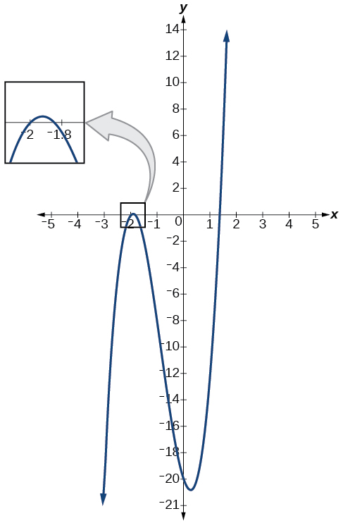
The graph of the polynomial function \(f(x)=4x^3+10x^2−6x−20\) in Figure \(\PageIndex{2}\) shows a zero at \(x=k=−2\). This confirms that \(x+2\) is a factor of \(4x^3+10x^2−6x−20\).

Figure \(\PageIndex{2}\)

Example \(\PageIndex{5}\): Using Synthetic Division to Divide a Fourth-Degree Polynomial

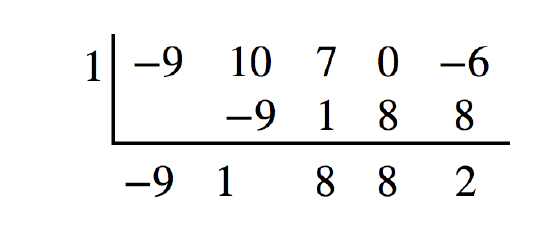
Use synthetic division to divide \(−9x^4+10x^3+7x^2−6\) by \(x−1\).

Solution

Notice there is no \(x\)-term. We will use a zero as the coefficient for that term.

The result is \(−9x^3+x^2+8x+8+\frac{2}{x−1}\).

\(\PageIndex{2}\)

Use synthetic division to divide \(3x^4+18x^3−3x+40\) by \(x+7\).

Solution

\(3x^3−3x^2+21x−150+\frac{1,090}{x+7}\)

Using Polynomial Division to Solve Application Problems

Polynomial division can be used to solve a variety of application problems involving expressions for area and volume. We looked at an application at the beginning of this section. Now we will solve that problem in the following example.

Example \(\PageIndex{6}\): Using Polynomial Division in an Application Problem

The volume of a rectangular solid is given by the polynomial \(3x^4−3x^3−33x^2+54x\). The length of the solid is given by \(3x\) and the width is given by \(x−2\). Find the height of the solid.

Solution

There are a few ways to approach this problem. We need to divide the expression for the volume of the solid by the expressions for the length and width. Let us create a sketch as in Figure \(\PageIndex{3}\).

Figure \(\PageIndex{3}\)

We can now write an equation by substituting the known values into the formula for the volume of a rectangular solid.

\[\begin{align*} V&=l{\cdot}w{\cdot}h \\ 3x^4−3x^3−33x^2+54x&=3x{\cdot}(x−2){\cdot}h \end{align*}\]

To solve for \(h\), first divide both sides by \(3x\).

\[\dfrac{3x{\cdot}(x−2){\cdot}h}{3x}=\dfrac{3x^4−3x^3−33x^2+54x}{3x} \nonumber\]

\[(x-2)h=\dfrac{x^3-x^2-11x+18}{x-2} \nonumber\]

Now solve for \(h\) using synthetic division.

\[h=\dfrac{x^3−x^2−11x+18}{x−2} \nonumber\]

\[{\begin{array}{c}-2\\ \\ \\ \end{array}}{\begin{align*}&\\[0pt]&{\begin{array}{r|}\\[0pt] \\[0pt] \end{array}}\\[1pt]& \\[2pt]& \end{align*}}\!\!
{\begin{array}{rrrr}
1 & -1 & -11 & 18\\
& 2 & 2 & -18 \\
\hline 1 & 1& -9 & 0
\end{array}}
\]

The quotient is \(x^2+x−9\) and the remainder is 0. The height of the solid is \(x^2+x−9\).

\(\PageIndex{3}\)

The area of a rectangle is given by \(3x^3+14x^2−23x+6\). The width of the rectangle is given by \(x+6\). Find an expression for the length of the rectangle.

Solution

\(3x^2−4x+1\)

Key Equations

Division Algorithm \(f(x)=d(x)q(x)+r(x)\) where \(q(x){\neq}0\)

Key Concepts

• Polynomial long division can be used to divide a polynomial by any polynomial with equal or lower degree.
• The Division Algorithm tells us that a polynomial dividend can be written as the product of the divisor and the quotient added to the remainder.
• Synthetic division is a shortcut that can be used to divide a polynomial by a binomial in the form x−k.
• Polynomial division can be used to solve application problems, including area and volume.

Footnotes

1 National Park Service. "Lincoln Memorial Building Statistics." http://www.nps.gov/linc/historycultu...statistics.htm. Accessed 4/3/2014

Glossary

Division Algorithm

given a polynomial dividend \(f(x)\) and a non-zero polynomial divisor \(d(x)\) where the degree of \(d(x)\) is less than or equal to the degree of \(f(x)\), there exist unique polynomials \(q(x)\) and \(r(x)\) such that \(f(x)=d(x)q(x)+r(x)\) where \(q(x)\) is the quotient and \(r(x)\) is the remainder. The remainder is either equal to zero or has degree strictly less than \(d(x)\).

synthetic division

a shortcut method that can be used to divide a polynomial by a binomial of the form \(x−k\)

Contributors

• Jay Abramson (Arizona State University) with contributing authors. Textbook content produced by OpenStax College is licensed under a Creative Commons Attribution License 4.0 license. Download for free at https://openstax.org/details/books/precalculus.