11.3: Application of Normal Distributions

Last updated
Save as PDF

Page ID: 109923

$ \newcommand{\vecs}[1]{\overset { \scriptstyle \rightharpoonup} {\mathbf{#1}} } $ $ \newcommand{\vecd}[1]{\overset{-\!-\!\rightharpoonup}{\vphantom{a}\smash {#1}}} $$\newcommand{\id}{\mathrm{id}}$ $ \newcommand{\Span}{\mathrm{span}}$ $ \newcommand{\kernel}{\mathrm{null}\,}$ $ \newcommand{\range}{\mathrm{range}\,}$ $ \newcommand{\RealPart}{\mathrm{Re}}$ $ \newcommand{\ImaginaryPart}{\mathrm{Im}}$ $ \newcommand{\Argument}{\mathrm{Arg}}$ $ \newcommand{\norm}[1]{\| #1 \|}$ $ \newcommand{\inner}[2]{\langle #1, #2 \rangle}$ $ \newcommand{\Span}{\mathrm{span}}$ $\newcommand{\id}{\mathrm{id}}$ $ \newcommand{\Span}{\mathrm{span}}$ $ \newcommand{\kernel}{\mathrm{null}\,}$ $ \newcommand{\range}{\mathrm{range}\,}$ $ \newcommand{\RealPart}{\mathrm{Re}}$ $ \newcommand{\ImaginaryPart}{\mathrm{Im}}$ $ \newcommand{\Argument}{\mathrm{Arg}}$ $ \newcommand{\norm}[1]{\| #1 \|}$ $ \newcommand{\inner}[2]{\langle #1, #2 \rangle}$ $ \newcommand{\Span}{\mathrm{span}}$$\newcommand{\AA}{\unicode[.8,0]{x212B}}$

Learning Objectives

Apply the characteristics of a normal distribution to solving applications.

Introduction

The normal distribution is the foundation for statistical inference and will be an essential part of many of those topics in later chapters. In the meantime, this section will cover some of the types of questions that can be answered using the properties of a normal distribution. The first examples deal with more theoretical questions that will help you master basic understandings and computational skills, while the later problems will provide examples with real data, or at least a real context.

Normal Distributions with Real Data

The foundation of performing experiments by collecting surveys and samples is most often based on the normal distribution, as you will learn in greater detail in later chapters. Here are two examples to get you started.

Example $\PageIndex{1}$

The Information Centre of the National Health Service in Britain collects and publishes a great deal of information and statistics on health issues affecting the population. One such comprehensive data set tracks information about the health of children [1]. According to its statistics, in 2006, the mean height of 12-year-old boys was 152.9 cm, with a standard deviation estimate of approximately 8.5 cm. (These are not the exact figures for the population, and in later chapters, we will learn how they are calculated and how accurate they may be, but for now, we will assume that they are a reasonable estimate of the true parameters.) If 12-year-old Cecil is 158 cm, approximately what percentage of all 12-year-old boys in Britain is he taller than?

Solution

We first must assume that the height of 12-year-old boys in Britain is normally distributed, and this seems like a reasonable assumption to make. As always, draw a sketch and estimate a reasonable answer prior to calculating the percentage. In this case, let’s use the calculator to sketch the distribution and the shading. First, decide on an appropriate window that includes about 3 standard deviations on either side of the mean. In this case, 3 standard deviations is about 25.5 cm, so add and subtract this value to/from the mean to find the horizontal extremes. Then enter the appropriate ‘ShadeNorm(’ command as shown:

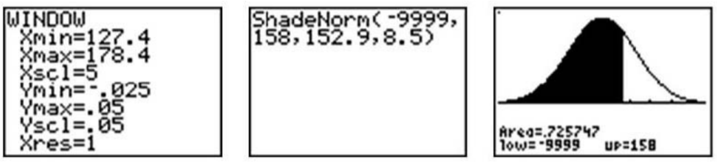
$clipboard_ea2de19631e6c6d042f33324468b468f6.png$

From this data, we would estimate that Cecil is taller than about 73% of 12-year-old boys. We could also phrase our assumption this way: the probability of a randomly selected British 12- year-old boy being shorter than Cecil is about 0.73. Often with data like this, we use percentiles. We would say that Cecil is in the 73^rd percentile for height among 12-year-old boys in Britain.

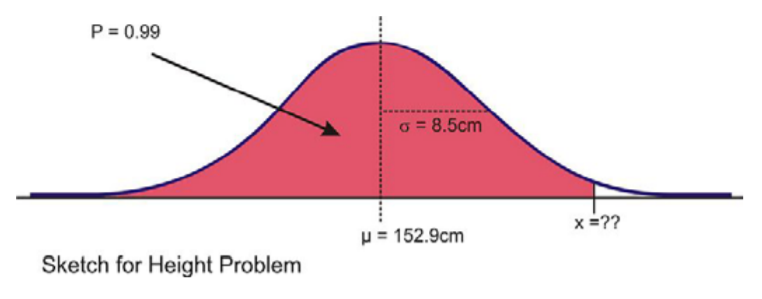
How tall would Cecil need to be in order to be in the top 1% of all 12-year-old boys in Britain?

Here is a sketch:

$clipboard_e93f4476074cf7de45d15e4ffe57a7bad.png$

In this case, we are given the percentage, so we need to use the ‘invNorm(’ command as shown.

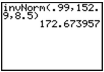
$clipboard_ee5bb0c07ef2ecd200d45fc9803774eff.png$

Our results indicate that Cecil would need to be about 173 cm tall to be in the top 1% of 12-year-old boys in Britain.

Example $\PageIndex{2}$

Suppose that the distribution of the masses of female marine iguanas in Puerto Villamil in the Galapagos Islands is approximately normal, with a mean mass of 950 g and a standard deviation of 325 g. There are very few young marine iguanas in the populated areas of the islands, because feral cats tend to kill them. How rare is it that we would find a female marine iguana with a mass less than 400 g in this area?

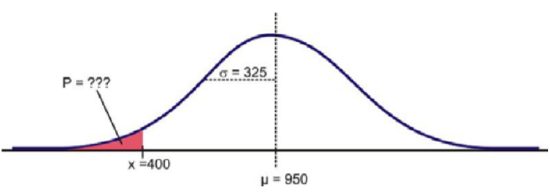
$clipboard_e70e5ac6ed5d7f52ce6681e5fd026d14f.png$

Solution

Using a graphing calculator, we can approximate the probability of a female marine iguana being less than 400 grams as follows:

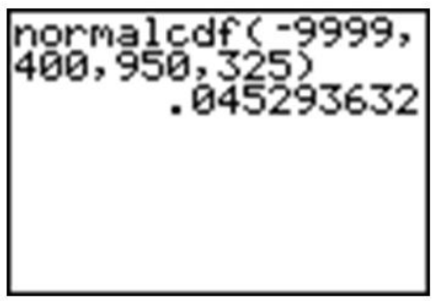
$clipboard_e03e8f50576994b74fe45b3d86a9ee483.png$

With a probability of approximately 0.045, or only about 5%, we could say it is rather unlikely that we would find an iguana this small.

Example $\PageIndex{3}$

The physical plant at the main campus of a large state university receives daily requests to replace florescent lightbulbs. The distribution of the number of daily requests is bell-shaped and has a mean of 59 and a standard deviation of 9. Using the Empirical rule, what is the approximate percentage of lightbulb replacement requests numbering between 59 and 77?

Solution

Since we want to use the Empirical Rule, we should draw a figure reflecting the Empirical Rule given the mean is $59$ and the standard deviation is $9$. Recall, 1 standard deviation from the mean is $59 ± 9$, two standard deviations from the mean is $59 ± 2 \cdot 9$, and 3 standard deviations from the mean is $59 ± 3 \cdot 9$.

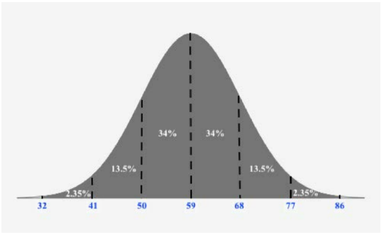
$clipboard_e634bf25b62ee508dfce32f906e0147ba.png$

Once we make this figure, we can easily the percentage of lightbulb replacement requests numbering between 59 and 77:

$34 \% + 13.5 \% = 47.5 \%$

Thus, $47.5 \%$ of lightbulb replacement requests numbering between 59 and 77.

Example $\PageIndex{4}$

A company has a policy of retiring company cars; this policy looks at number of miles driven, purpose of trips, style of car and other features. The distribution of the number of months in service for the fleet of cars is bell-shaped and has a mean of 41 months and a standard deviation of 5 months. Using the Empirical Rule, what is the approximate percentage of cars that remain in service between 46 and 56 months?

Solution

Since we want to use the Empirical Rule, we should draw a figure reflecting the Empirical Rule given the mean is 41 and the standard deviation is 5:

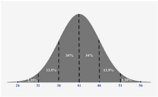
$clipboard_ecec6a8748e19e47ad4369f12031cb4e3.png$

Once we make this figure, we can easily the approximate percentage of cars that remain in service between 46 and 56 months:

$13.5 \% + 2.35 \% = 15.85 \%$

Thus, $15.85 \%$ of cars remain in service between 46 and 56 months.

Exercises

1. Which of the following intervals contains the middle 95% of the data in a standard normal distribution?

a) $z < 2$

b) $z ≤ 1.645$

c) $z ≤ 1.96$

d) $−1.645 ≤ z ≤ 1.645$

e) $−1.96 ≤ z ≤ 1.96$

2. The manufacturing process at a metal-parts factory produces some slight variation in the diameter of metal ball bearings. The quality control experts claim that the bearings produced have a mean diameter of 1.4 cm. If the diameter is more than 0.0035 cm too wide or too narrow, they will not work properly. In order to maintain its reliable reputation, the company wishes to ensure that no more than one-tenth of 1% of the bearings that are made are ineffective. What would the standard deviation of the manufactured bearings need to be in order to meet this goal?

3. Suppose that the wrapper of a certain candy bar lists its weight as 2.13 ounces. Naturally, the weights of individual bars vary somewhat. Suppose that the weights of these candy bars vary according to a normal distribution, with $µ = 2.2$ ounces and $σ = 0.04$ ounces.

a) What proportion of the candy bars weigh less than the advertised weight?

b) What proportion of the candy bars weight between 2.2 and 2.3 ounces?

c) A candy bar of what weight would be heavier than all but 1% of the candy bars out there?

d) If the manufacturer wants to adjust the production process so that no more than 1 candy bar in 1000 weighs less than the advertised weight, what would the mean of the actual weights need to be? (Assume the standard deviation remains the same.)

e) If the manufacturer wants to adjust the production process so that the mean remains at 2.2 ounces and no more than 1 candy bar in 1000 weighs less than the advertised weight, how small does the standard deviation of the weights need to be?

4. The Acme Company manufactures widgets. The distribution of widget weights is bell-shaped. The widget weights have a mean of 51 ounces and a standard deviation of 4 ounces. Use the Empirical Rule to answer the following questions.

a) 99.7% of the widget weights lie between what two weights?

b) What percentage of the widget weights lie between 43 and 63 ounces?

c) What percentage of the widget weights lie above 47?

Standard Normal Table Area under the Normal Curve from 0 to z $clipboard_ee8d9b2dd27d551a2fe3bc41fe72d9b3c.png$
z	0.00	0.01	0.02	0.03	0.04	0.05	0.06	0.07	0.08	0.09
0.00	0.00000	0.00399	0.00798	0.01197	0.01595	0.01994	0.02392	0.02790	0.03188	0.03586
0.10	0.03983	0.04380	0.04776	0.05172	0.05567	0.05962	0.06356	0.06749	0.07142	0.07535
0.20	0.07926	0.08317	0.08706	0.09095	0.09483	0.09871	0.10257	0.10642	0.11026	0.11409
0.30	0.11791	0.12172	0.12552	0.12930	0.13307	0.13683	0.14058	0.14431	0.14803	0.15173
0.40	0.15542	0.15910	0.16276	0.16640	0.17003	0.17364	0.17724	0.18082	0.18439	0.18793
0.50	0.19146	0.19497	0.19847	0.20194	0.20540	0.20884	0.21226	0.21566	0.21904	0.22240
0.60	0.22575	0.22907	0.23237	0.23565	0.23891	0.24215	0.24537	0.24857	0.25175	0.25490
0.70	0.25804	0.26115	0.26424	0.26730	0.27035	0.27337	0.27637	0.27935	0.28230	0.28524
0.80	0.28814	0.29103	0.29389	0.29673	0.29955	0.30234	0.30511	0.30785	0.31057	0.31327
0.90	0.31594	0.31859	0.32121	0.32381	0.32639	0.32894	0.33147	0.33398	0.33646	0.33891
1.00	0.34134	0.34375	0.34614	0.34849	0.35083	0.35314	0.35543	0.35769	0.35993	0.36214
1.10	0.36433	0.36650	0.36864	0.37076	0.37286	0.37493	0.37698	0.37900	0.38100	0.38298
1.20	0.38493	0.38686	0.38877	0.39065	0.39251	0.39435	0.39617	0.39796	0.39973	0.40147
1.30	0.40320	0.40490	0.40658	0.40824	0.40988	0.41149	0.41308	0.41466	0.41621	0.41774
1.40	0.41924	0.42073	0.42220	0.42364	0.42507	0.42647	0.42785	0.42922	0.43056	0.43189
1.50	0.43319	0.43448	0.43574	0.43699	0.43822	0.43943	0.44062	0.44179	0.44295	0.44408
1.60	0.44520	0.44630	0.44738	0.44845	0.44950	0.45053	0.45154	0.45254	0.45352	0.45449
1.70	0.45543	0.45637	0.45728	0.45818	0.45907	0.45994	0.46080	0.46164	0.46246	0.46327
1.80	0.46407	0.46485	0.46562	0.46638	0.46712	0.46784	0.46856	0.46926	0.46995	0.47062
1.90	0.47128	0.47193	0.47257	0.47320	0.47381	0.47441	0.47500	0.47558	0.47615	0.47670
2.00	0.47725	0.47778	0.47831	0.47882	0.47932	0.47982	0.48030	0.48077	0.48124	0.48169
2.10	0.48214	0.48257	0.48300	0.48341	0.48382	0.48422	0.48461	0.48500	0.48537	0.48574
2.20	0.48610	0.48645	0.48679	0.48713	0.48745	0.48778	0.48809	0.48840	0.48870	0.48899
2.30	0.48928	0.48956	0.48983	0.49010	0.49036	0.49061	0.49086	0.49111	0.49134	0.49158
2.40	0.49180	0.49202	0.49224	0.49245	0.49266	0.49286	0.49305	0.49324	0.49343	0.49361
2.50	0.49379	0.49396	0.49413	0.49430	0.49446	0.49461	0.49477	0.49492	0.49506	0.49520
2.60	0.49534	0.49547	0.49560	0.49573	0.49585	0.49598	0.49609	0.49621	0.49632	0.49643
2.70	0.49653	0.49664	0.49674	0.49683	0.49693	0.49702	0.49711	0.49720	0.49728	0.49736
2.80	0.49744	0.49752	0.49760	0.49767	0.49774	0.49781	0.49788	0.49795	0.49801	0.49807
2.90	0.49813	0.49819	0.49825	0.49831	0.49836	0.49841	0.49846	0.49851	0.49856	0.49861
3.00	0.49865	0.49869	0.49874	0.49878	0.49882	0.49886	0.49889	0.49893	0.49896	0.49900
3.10	0.49903	0.49906	0.49910	0.49913	0.49916	0.49918	0.49921	0.49924	0.49926	0.49929
3.20	0.49931	0.49934	0.49936	0.49938	0.49940	0.49942	0.49944	0.49946	0.49948	0.49950
3.30	0.49952	0.49953	0.49955	0.49957	0.49958	0.49960	0.49961	0.49962	0.49964	0.49965
3.40	0.49966	0.49968	0.49969	0.49970	0.49971	0.49972	0.49973	0.49974	0.49975	0.49976
3.50	0.49977	0.49978	0.49978	0.49979	0.49980	0.49981	0.49981	0.49982	0.49983	0.49983
3.60	0.49984	0.49985	0.49985	0.49986	0.49986	0.49987	0.49987	0.49988	0.49988	0.49989
3.70	0.49989	0.49990	0.49990	0.49990	0.49991	0.49991	0.49992	0.49992	0.49992	0.49992
3.80	0.49993	0.49993	0.49993	0.49994	0.49994	0.49994	0.49994	0.49995	0.49995	0.49995
3.90	0.49995	0.49995	0.49996	0.49996	0.49996	0.49996	0.49996	0.49996	0.49997	0.49997
4.00	0.49997	0.49997	0.49997	0.49997	0.49997	0.49997	0.49998	0.49998	0.49998	0.49998

Search

Learning Objectives

Introduction

Normal Distributions with Real Data

Example \(\PageIndex{1}\)

Example \(\PageIndex{2}\)

Example \(\PageIndex{3}\)

Example \(\PageIndex{4}\)

Exercises