

17.1: The Basics of Exponential Functions
- Page ID
- 174381
\( \newcommand{\vecs}[1]{\overset { \scriptstyle \rightharpoonup} {\mathbf{#1}} } \)
\( \newcommand{\vecd}[1]{\overset{-\!-\!\rightharpoonup}{\vphantom{a}\smash {#1}}} \)
\( \newcommand{\dsum}{\displaystyle\sum\limits} \)
\( \newcommand{\dint}{\displaystyle\int\limits} \)
\( \newcommand{\dlim}{\displaystyle\lim\limits} \)
\( \newcommand{\id}{\mathrm{id}}\) \( \newcommand{\Span}{\mathrm{span}}\)
( \newcommand{\kernel}{\mathrm{null}\,}\) \( \newcommand{\range}{\mathrm{range}\,}\)
\( \newcommand{\RealPart}{\mathrm{Re}}\) \( \newcommand{\ImaginaryPart}{\mathrm{Im}}\)
\( \newcommand{\Argument}{\mathrm{Arg}}\) \( \newcommand{\norm}[1]{\| #1 \|}\)
\( \newcommand{\inner}[2]{\langle #1, #2 \rangle}\)
\( \newcommand{\Span}{\mathrm{span}}\)
\( \newcommand{\id}{\mathrm{id}}\)
\( \newcommand{\Span}{\mathrm{span}}\)
\( \newcommand{\kernel}{\mathrm{null}\,}\)
\( \newcommand{\range}{\mathrm{range}\,}\)
\( \newcommand{\RealPart}{\mathrm{Re}}\)
\( \newcommand{\ImaginaryPart}{\mathrm{Im}}\)
\( \newcommand{\Argument}{\mathrm{Arg}}\)
\( \newcommand{\norm}[1]{\| #1 \|}\)
\( \newcommand{\inner}[2]{\langle #1, #2 \rangle}\)
\( \newcommand{\Span}{\mathrm{span}}\) \( \newcommand{\AA}{\unicode[.8,0]{x212B}}\)
\( \newcommand{\vectorA}[1]{\vec{#1}} % arrow\)
\( \newcommand{\vectorAt}[1]{\vec{\text{#1}}} % arrow\)
\( \newcommand{\vectorB}[1]{\overset { \scriptstyle \rightharpoonup} {\mathbf{#1}} } \)
\( \newcommand{\vectorC}[1]{\textbf{#1}} \)
\( \newcommand{\vectorD}[1]{\overrightarrow{#1}} \)
\( \newcommand{\vectorDt}[1]{\overrightarrow{\text{#1}}} \)
\( \newcommand{\vectE}[1]{\overset{-\!-\!\rightharpoonup}{\vphantom{a}\smash{\mathbf {#1}}}} \)
\( \newcommand{\vecs}[1]{\overset { \scriptstyle \rightharpoonup} {\mathbf{#1}} } \)
\(\newcommand{\longvect}{\overrightarrow}\)
\( \newcommand{\vecd}[1]{\overset{-\!-\!\rightharpoonup}{\vphantom{a}\smash {#1}}} \)
\(\newcommand{\ket}[1]{\left| #1 \right>}\)
\(\newcommand{\bra}[1]{\left< #1 \right|}\)
\(\newcommand{\braket}[2]{\left< #1 \vphantom{#2} \right| \left. #2 \vphantom{#1} \right>}\)
\(\newcommand{\braopket}[3]{\left< #1 \vphantom{#2}\vphantom{#3} \right| #2 \vphantom{#1}\vphantom{#3} \left| #3 \vphantom{#1}\vphantom{#2} \right>}\)
\(\newcommand{\qmvec}[1]{\mathbf{\vec{#1}}}\)
\(\newcommand{\op}[1]{\hat{\mathbf{#1}}}\)
\(\newcommand{\expect}[1]{\langle #1 \rangle}\)
\(\newcommand{\dfn}[1]{\emph{\textbf{#1}}}\)
Videos
Lecture (level = intermediate algebra): An Introduction to Exponential Functions
Lecture (level = intermediate algebra): Creating Exponential Functions from Applications
Review (level = college algebra): The Basics of Exponential Functions
Review (level = college algebra): Types of Exponential Growth and Decay
Definitions and Theorems
For an exponential function with base \( b \), every increase of 1 in input results in multiplying the previous function value by \( b \). This is called the base multiplier property.
An exponential function is a function with the form\[f(x)=a b^x, \nonumber \]where \(a\) is a non-zero real number called the initial value and \(b\) is any positive real number, called the base, such that \(b \neq 1\). This function is also referred to as the exponential function base \( b \).
The base is required to be positive so that \(b^x\) is defined for every real number \(x\); for a negative base, an expression such as \((-4)^{1/2}\) has no real value. The base is also excluded from equaling \(1\), because \(1^x=1\) for all \(x\), which produces the constant function \(f(x)=a\) rather than an exponential one.
The expression \(ab^x\) means \(a\cdot(b^x)\), not \((ab)^x\). By the order of operations, the exponent \(x\) applies only to the base \(b\); the coefficient \(a\) is multiplied afterward. For example, \(2\cdot 3^2=2\cdot 9=18\), whereas \((2\cdot 3)^2=6^2=36\).
Let \( f(x) =a b^x \), with \( a \gt 0 \), \(b \gt 0\), and \(b \neq 1\):
- The domain of \(f\) is all real numbers.
- The range of \(f\) is all positive real numbers.
- The \( y \)-intercept is \(( 0,a )\).
- The graph of \( f \) includes the point \( (1,ab) \).
- The horizontal asymptote is \(y=0\).
- If \( b > 1 \),
- \( f \) is increasing,
- as \( x \to -\infty \), \( f(x) \to 0 \), and
- as \( x \to \infty \), \( f(x) \to \infty \).
- If \( 0 < b < 1 \),
- \( f(x) \) is decreasing,
- as \( x \to -\infty \), \( f(x) \to \infty \), and
- as \( x \to \infty \), \( f(x) \to 0 \).
A function that models exponential growth or exponential decay grows or decays by a rate proportional to the amount present. For any real number \(t\) and any positive real numbers \(P_0\) and \(b\) such that \(b \neq 1\), an exponential growth or decay function has the form\[P(t)=P_0 \, b^t, \nonumber \]where
- \(P_0\) is the initial or starting value of the function, and
- \(b\) is the growth or decay factor
- if \( b > 1 \), it is a growth factor or growth multiplier per unit \(t\)
- if \( 0 < b < 1 \), it is a decay factor or decay multiplier per unit \( t \).
If \(f(x)=ab^x\), then\[f(x+1)=b\cdot f(x)\nonumber\]for every real number \(x\). That is, increasing the input by \(1\) multiplies the output by the base \(b\).

The base controls the long-run behavior of the graph. When \(b\gt 1\), the outputs increase without bound as \(x\to\infty\) and shrink toward \(0\) as \(x\to-\infty\), so the curve hugs the \(x\)-axis on the left and rises steeply on the right. When \(0\lt b\lt 1\), the roles reverse: the outputs shrink toward \(0\) as \(x\to\infty\) and grow without bound as \(x\to-\infty\). In either case the graph approaches, but never reaches, the horizontal asymptote \(y=0\). If instead \(a\lt 0\), the graph is reflected across the \(x\)-axis (its range becomes \((-\infty,0)\)), but \(y=0\) remains the horizontal asymptote.
Examples
Let \(f(x)=2\cdot 3^x\). Find \(f(-1)\), \(f(0)\), \(f(1)\), and \(f(3)\).
- Solution
-
Substitute each input into \(f(x)=2\cdot 3^x\) and simplify, recalling that \(3^{-1}=\frac{1}{3}\) and \(3^0=1\).
\[f(-1)=2\cdot 3^{-1}=\dfrac{2}{3},\qquad f(0)=2\cdot 3^{0}=2,\nonumber\] \[f(1)=2\cdot 3^{1}=6,\qquad f(3)=2\cdot 3^{3}=2\cdot 27=54.\nonumber\]
Determine whether each function models exponential growth or exponential decay, and identify its base.
- \(f(x)=4\cdot 2^x\)
- \(f(x)=3\cdot\left(\frac{1}{2}\right)^x\)
- \(f(x)=7\cdot\left(\frac{5}{4}\right)^x\)
- Solutions
-
Read the base directly from the form \(ab^x\) and compare it to \(1\).
- The base is \(b=2\). Since \(2\gt 1\), the function models exponential growth.
- The base is \(b=\frac{1}{2}\). Since \(0\lt\frac{1}{2}\lt 1\), the function models exponential decay.
- The base is \(b=\frac{5}{4}\). Since \(\frac{5}{4}\gt 1\), the function models exponential growth.
For \(f(x)=6\cdot\left(\frac{1}{4}\right)^x\), state the \(y\)-intercept and the horizontal asymptote, and determine whether the function models growth or decay.
- Solution
-
The \(y\)-intercept occurs at \(x=0\). Since \(\left(\frac{1}{4}\right)^0=1\), we have \(f(0)=6\cdot 1=6\), so the \(y\)-intercept is \((0,6)\), matching the coefficient \(a=6\).
Every function of the form \(ab^x\) with \(a\gt 0\) has the horizontal asymptote \(y=0\); as \(x\to\infty\) the outputs approach \(0\) here, so the asymptote is \(y=0\).
The base is \(b=\frac{1}{4}\), and since \(0\lt\frac{1}{4}\lt 1\), the function models exponential decay.
Let \(f(x)=5\cdot\left(\frac{1}{2}\right)^x\). Find \(f(-2)\), \(f(0)\), \(f(2)\), and \(f(3)\).
- Solution
-
Substitute each input, using \(\left(\frac{1}{2}\right)^{-2}=2^{2}=4\) for the negative exponent.
\[f(-2)=5\cdot\left(\dfrac{1}{2}\right)^{-2}=5\cdot 4=20,\qquad f(0)=5\cdot\left(\dfrac{1}{2}\right)^{0}=5,\nonumber\] \[f(2)=5\cdot\left(\dfrac{1}{2}\right)^{2}=\dfrac{5}{4},\qquad f(3)=5\cdot\left(\dfrac{1}{2}\right)^{3}=\dfrac{5}{8}.\nonumber\]The outputs shrink as \(x\) increases, as expected for a decay function.
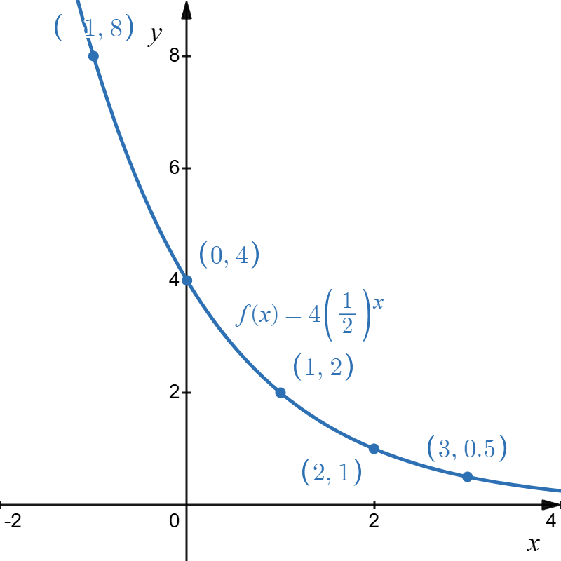
Complete a table of values for \(f(x)=4\cdot\left(\frac{1}{2}\right)^x\) at \(x=-1,0,1,2,3\), sketch its graph, and describe its behavior.
- Solution
-
Evaluate the function at each input to build the table.
\(x\) \(f(x)\) \((x,f(x))\) \(-1\) \(8\) \((-1,8)\) \(0\) \(4\) \((0,4)\) \(1\) \(2\) \((1,2)\) \(2\) \(1\) \((2,1)\) \(3\) \(\dfrac{1}{2}\) \(\left(3,\dfrac{1}{2}\right)\) 
Figure \(\PageIndex{2}\): The graph of \(f(x)=4\left(\tfrac{1}{2}\right)^x\), decreasing toward the horizontal asymptote \(y=0\). Because the base is \(\frac{1}{2}\), each increase of \(1\) in \(x\) multiplies the output by \(\frac{1}{2}\)—that is, it halves the output. The function is decreasing, models exponential decay, and its graph approaches the horizontal asymptote \(y=0\) as \(x\to\infty\) without ever reaching it.
An exponential function \(f(x)=ab^x\) passes through the points \((0,3)\) and \((2,27)\). Find \(a\) and \(b\), then write the function.
- Solution
-
Use the point \((0,3)\) first, since it isolates the coefficient. Substituting \(x=0\) gives\[f(0)=a\cdot b^{0}=a=3,\nonumber\]so \(a=3\).
Now use the point \((2,27)\) with \(a=3\):\[f(2)=3\cdot b^{2}=27\quad\Longrightarrow\quad b^{2}=9\quad\Longrightarrow\quad b=3.\nonumber\]We take \(b=3\) rather than \(b=-3\), because the base of an exponential function must be positive.
Therefore, \(f(x)=3\cdot 3^x\).
MyOpenMath Practice
Sources
Several parts of this text use modifications from the following sources:
- Wikipedia article: "Exponential function"
- Wikipedia article: "Exponential growth"
All of these sources are released under the Creative Commons Attribution-Share-Alike License 4.0.