1.2: Graphical Investigation of Limits

Section Preview

Note to the Instructor (click to expand)

This section is essentially a repeat of the previous section but from the graphical perspective. It will be important to let the student know that this method of investigating limits is only slightly better than numerical investigations.

Core Prerequisites (i.e., "Understanding the Lesson"): The following prerequisite topics (which have not already been listed as prerequisites in previous sections of this text) are required to understand the core concepts in this lesson.

(click to expand)

• Graphs
  • The Cartesian Coordinate System and the Quadrants
  • Reading Values from Graphs
• Rational Functions
  • Asymptotes
• Logarithmic Functions
  • Graphing Logarithmic Functions
• Trigonometry
  • Base Graphs of the Trigonometric Functions

Operational Prerequisites (i.e., "Completing the Homework"): The following prerequisite topics (which have not already been listed as prerequisites in previous sections of this text) are needed to complete the homework.

(click to expand)

• Arithmetic
  • Mathematical Operations — Addition, Subtraction, Multiplication, and Division
• Trigonometry
  • Trigonometric Identities — The Reciprocal and Ratio Identities

The following is a list of learning objectives for this section.

Learning Objectives (click to expand)

• Describe the limit of a function and use proper limit notation.
• Use a graph to estimate a function's limit or identify when the limit does not exist.
• Investigate one-sided limits.
• Using correct notation, describe an infinite limit.
• Define a vertical asymptote in terms of limits.
• Determine the value of a limit near a vertical asymptote conceptually.

We began our exploration of limits by numerically investigating the functions \(f(x)=\frac{x^2-4}{x-2}\), \(g(x)=\frac{|x-2|}{x-2}\), and \(h(x)=\frac{1}{(x-2)^2}\). We now continue this investigation from a new perspective by looking at the graphs of these function, which are shown in Figure \(\PageIndex{1}\). In particular, let's focus our attention on the behavior of each graph at and around \(x=2\).

Figure \(\PageIndex{1}\): These graphs show the behavior of three different functions around \(x=2\).

Each of the three functions is undefined at \(x=2\), but if we make this statement and no other, we give an incomplete picture of how each function behaves in the vicinity of \(x=2\). To express the behavior of each graph in the vicinity of \(2\) more thoroughly, we need to use the concept of a limit.

Finite Limit at a Finite Number - The Graphical Approach

Let's first take a closer look at Figure \(\PageIndex{1a}\) and how the function \(f(x)= \frac{x^2-4}{x-2}\) behaves around \(x=2\). As the values of \(x\) approach \(2\) from either side of \(2\), the values of \(y=f(x)\) approach \(4\). As we did when investigating limits numerically, we say that the limit of \(f(x)\) as \(x\) approaches \(2\) is \(4\). Again, we express this symbolically as\[\lim_{x \to 2} f(x)=4.\nonumber\]With graphical explorations of limits, it's even more important to repeat our caution from last section.

Caution: \(x \neq a\)

The intuitive definition of a finite limit at a finite number states that \(x\) need not equal \(a\). This is critical to understand. The \(x\)-values are allowed to get very close to \(a\) but will never become \(a\). In a very real sense, the limit,\[\lim_{x \to a} f(x)=L,\nonumber\]is concerned with the function values as \(x\) gets closer and closer to \(a\); however, it is not asking, "What is \(f(a)\)?" In fact, it could be the case that \(f(a)\) does not exist or \(L \neq f(a)\).

Interactive Element: A Limit at a Hole

The following Interactive Element might help you visualize how a limit can exist even where the function is undefined.

Interact: Drag the red point along the curve toward \(x = 2\) from the left, then from the right.

Observation: As \(x \to 2\) from either side, \(y\) approaches \(4\), so \(\lim_{x \to 2} f(x) = 4\) — even though the open circle shows \(f(2)\) is undefined.

We mentioned the issues with investigating limits numerically in the previous section. Graphical investigations are only slightly less dangerous. In practice, using a graph to state the value of a limit presents three issues:

1. if not given a graph, then it could be arduous (or impossible) to recreate the graph of the function, and
2. graphs can be visually "tricky," leading you to assume a function behavior that is not actually present.

These warnings stated, we still take the time to investigate limits graphically in order to gain an intuitive understanding of limits.

Using Graphs to Estimate Limits

Example \(\PageIndex{1}\)

We built a table in the previous section to conjecture that\[\lim_{\theta \to 0}\frac{\sin \theta}{\theta} = 1.\nonumber\]Verify the value of this limit by graphing \(y = \frac{\sin \theta}{\theta}\) near to \(x = 0\).

Solution

A Desmos-generated graph of \(f(\theta)=\frac{\sin \theta}{\theta}\) is shown in Figure \(\PageIndex{2}\), and it supports our estimate. We can see that the function values look to be tending to a value of 1 as \(x \to 0\) from both the left and the right.

Figure \(\PageIndex{2}\): The graph of \(f(t)=\frac{\sin \theta}{\theta}\) confirms the estimate from the previous section.

There are a few things we need to observe about Example \(\PageIndex{1}\).

First, recall the following caution from the last section.

Caution: Calculus Does Not Work in Degrees

For reasons we will discuss later, when working with trigonometric functions in Calculus, you must work in radians—not degrees.

If you attempted Example \(\PageIndex{1}\), but had a different graph, it is highly likely your calculator was set to degree mode. Do yourself a favor and set it to radian mode for the rest of Calculus—you will have one less thing to worry about as you adventure through the Calculus series.

The second observation also centers on something I included in Figure \(\PageIndex{2}\) that your graph would likely not have included—the open circle at \(\left( 0,1 \right)\). How did my graph show that and your didn't? Well, truthfully, my graph looked like your to begin with. That is, it didn't show that the given function wasn't defined at \(\theta = 0\). This is why graphs can be deceiving! Luckily, I only wanted to know the behavior of the graph near to \(\theta = 0\). Since the function had the obvious domain issue at \(\theta = 0\), I manually placed an open circle on the graph at \(\left( 0,1 \right)\).

Our next observation is more of a question: We can see in Figure \(\PageIndex{2}\) that the function, \(f(\theta) = \frac{\sin \theta}{\theta}\), is not defined at \(\theta = 0\). Why didn't we then say that the limit didn't exist?

Recall that \(\displaystyle \lim_{\theta \to 0} \frac{\sin \theta}{\theta}\), is concerned with \(\theta\) approaching \(0\)—not becoming \(0\). Thus, the function not existing at \(\theta = 0\) is not an issue. This is a common theme in Calculus and you must immediately come to terms with the reality that limits are unconcerned with the value of the function at the \(x\)-value they are approaching.

The final observation is yet another warning from the previous section—it looks like \(\displaystyle \lim_{\theta \to 0} \frac{\sin \theta}{\theta} = 1\); however, this is not a proof that the value of the limit is 1. For now, we only have two methods to evaluate limits (tables and graphs), so we will have to cross our fingers and hope we are not making too many assumptions. Luckily, we will eventually have analytical methods to determine the value of a limit precisely without the need for technology, tables, or graphs.

Example \(\PageIndex{2}\)

Verify\[\lim_{x \to 4}\frac{\sqrt{x}-2}{x-4} = 0.25\nonumber\]using a graph (this is another example from last section).

Solution

The graph of \(f(x)=\frac{\sqrt{x}-2}{x-4}\), shown in Figure \(\PageIndex{3}\), verifies our result from the previous section.

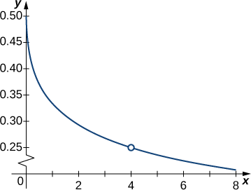
Figure \(\PageIndex{3}\): The graph of \(\frac{\sqrt{x}-2}{x-4}\) verifies the estimate from the previous section.

Checkpoint \(\PageIndex{2}\)

At this point, we see from Examples \(\PageIndex{1}\) and \(\PageIndex{2}\) that it may be just as easy, if not easier, to estimate a limit of a function by inspecting its graph (rather than building a table of function values). In Example \(\PageIndex{3}\), we evaluate a new limit (not from the previous section) exclusively by looking at a graph rather than by using a table of function values.

Example \(\PageIndex{3}\)

For \(g(x)\) shown in Figure \(\PageIndex{4}\) below, evaluate\[\lim_{x \to -1} g(x).\nonumber\]

Figure \(\PageIndex{4}\)

Solution

Despite the fact that \(g(-1) = 4\), as the \(x\)-values approach \(-1\) from either side, the corresponding values of \(g\) approach 3. Therefore,\[\lim_{x \to -1} g(x) = 3.\nonumber\]Note that we can determine this limit without even knowing the algebraic expression of the function.

Checkpoint \(\PageIndex{3}\)

Revisiting the Existence of a Limit

The next example graphically verifies a result from the previous section.

Example \(\PageIndex{4}\)

Evaluate\[\lim_{x \to 0}\sin\left(\dfrac{1}{x}\right)\nonumber\]using a graph.

Solution

The graph of \(f(x)=\sin(1/x)\) is shown in Figure \(\PageIndex{5}\), and it gives a clearer picture of the behavior of \(\sin(1/x)\) as \(x\) approaches \(0\). You can see that \(\sin(1/x)\) oscillates ever more wildly between \(-1\) and \(1\) as \(x\) approaches \(0\). Since this means the limit does not become a single value (finite or infinite), we can confidently assume that the limit DNE.

Figure \(\PageIndex{5}\): The graph of \(f(x)=\sin (1/x)\) oscillates rapidly between \(-1\) and \(1\) as \(x\) approaches \(0\).

Checkpoint \(\PageIndex{4}\)

Use a graph to evaluate\[\lim_{x \to 2}\dfrac{∣x^2-4∣}{x-2},\nonumber\]if possible.

Answer

\(\displaystyle \lim_{x \to 2}\frac{∣x^2-4∣}{x-2}\) does not exist.

Revisiting One-Sided Limits

As will all limits in this section, one-sided limits are much easier when you have the graph of the function at hand.

Example \(\PageIndex{5}\)

For the function\[f(x)=\begin{cases}x+1, & \text{if }x<2\\ x^2-4, & \text{if }x \geq 2 \end{cases},\nonumber\]evaluate each of the following limits by creating a graph of the function.

1. \(\displaystyle \lim_{x \to 2^-}f(x)\)
2. \(\displaystyle \lim_{x \to 2^+}f(x)\)

Solutions

Figure \(\PageIndex{6}\) shows a graph of \(f(x)\). We can see that as \(x \to 2^-\), the function values are climbing to \(y = 3\), and as \(x \to 2^+\), \(f(x) \to 0\). Therefore,\[\lim_{x \to 2^-}f(x) = 3 \quad \text{and} \quad\lim_{x \to 2^+}f(x) = 0.\nonumber\]

Figure \(\PageIndex{6}\): The graph of \(f(x)=\begin{cases}x+1, & \text{if }x<2\\ x^2-4, & \text{if }x \geq 2\end{cases}\) has a break at \(x=2\).

Interactive Element: When One-Sided Limits Disagree

The following Interactive Element might help you visualize why a limit fails to exist at a jump.

Interact: Drag the red point toward \(x = 2\) from the left, then approach \(x = 2\) again from the right.

Observation: From the left, \(y \to 3\); from the right, \(y \to 0\). Because the two one-sided limits disagree, \(\lim_{x \to 2} f(x)\) does not exist.

Revisiting Infinite Limits at Finite Numbers

Example \(\PageIndex{6}\)

Reevaluate each of the following limits from the previous section using a graph.

1. \(\displaystyle \lim_{x \to 0^-} \frac{1}{x}\)
2. \(\displaystyle \lim_{x \to 0^+} \frac{1}{x}\)
3. \(\displaystyle \lim_{x \to 0}\frac{1}{x}\)

Solutions

The graph of \(f(x)=1/x\) is shown in Figure \(\PageIndex{7}\) below. From this graph, we can see that \(\displaystyle \lim_{x \to 0^-} \frac{1}{x} = -\infty\), \(\displaystyle \lim_{x \to 0^+} \frac{1}{x} = \infty\), and, because the left- and right-hand limits do not match, \(\displaystyle \lim_{x \to 0}\frac{1}{x}\) DNE.

Figure \(\PageIndex{7}\): The graph of \(f(x)=1/x\) confirms that the limit as \(x\) approaches \(0\) does not exist.

We finally reach a moment in this section where we do something more than we did last section. The definition of an infinite limit at a finite number and some inspiration from Figure \(\PageIndex{7}\) allow us to formalize a concept from past courses.

Definition: Vertical Asymptote

The function \(f(x)\) is said to have a vertical asymptote at \(x = a\) if any of the following are true.\[\begin{array}{rcl} \displaystyle\lim_{x \to a^-}f(x) & = & +\infty\\ \displaystyle\lim_{x \to a^-}f(x) & = & -\infty\\ \displaystyle\lim_{x \to a^+}f(x) & = & +\infty\\ \displaystyle\lim_{x \to a^+}f(x) & = & -\infty \\ \displaystyle\lim_{x \to a}f(x) & = & +\infty\\ \displaystyle\lim_{x \to a}f(x) & = & -\infty\\ \end{array}\nonumber\]

Interactive Element: A Vertical Asymptote as an Infinite Limit

The following Interactive Element might help you visualize how an infinite limit produces a vertical asymptote.

Interact: Drag the orange point toward \(x = 2\) from the left, then from the right, and watch its height.

Observation: As \(x \to 2\) from either side, \(y\) grows without bound, so \(\lim_{x \to 2}\frac{1}{(x-2)^2} = +\infty\). An infinite limit like this is exactly what it means for the graph to have a vertical asymptote at \(x = 2\).

Checkpoint \(\PageIndex{6}\)

If possible, use a graph to evaluate each of the following limits and state whether the function has a vertical asymptote at \(x = 0\).

1. \(\displaystyle \lim_{x \to 0^-}\frac{1}{x^2}\)
2. \(\displaystyle \lim_{x \to 0^+}\frac{1}{x^2}\)
3. \(\displaystyle \lim_{x \to 0}\frac{1}{x^2}\)

Answers

1. \(\displaystyle \lim_{x \to 0^-}\frac{1}{x^2}=+\infty\)
2. \(\displaystyle \lim_{x \to 0^+}\frac{1}{x^2}=+\infty\)
3. \(\displaystyle \lim_{x \to 0}\frac{1}{x^2}=+\infty\)

From the fact that any of these limits (at the finite number \(x= 0\)) is infinite, we can state that \(f(x)\) has a vertical asymptote at \(x = 0\).

Conceptual Investigation of an Infinite Limit

When given a function that has a vertical asymptote at \(x = a\), a conceptual investigation of the limit as \(x\) approaches \(a\) can often be done. This type of investigation relies heavily on your mastery of the prerequisite knowledge to Calculus—specifically, domains of functions, vertical asymptotes, and the graphs of logarithmic and trigonometric functions.

Before getting too deep into conceptual investigations of infinite limits, we need to understand the nature of a ratio when its denominator is approaching zero.

Table \(\PageIndex{1}\): A comparison of ratios with denominators approaching zero

\(f(x) = \frac{1}{x}\)	\(g(x) = \frac{13}{x}\)	\(h(x) = -\frac{2}{x^2}\)
\(\frac{1}{0.1} = 10\)	\(\frac{13}{-0.1} =-130\)	\(-\frac{2}{(-0.1)^2} =-200\)
\(\frac{1}{0.01} = 100\)	\(\frac{13}{-0.01} =-1300\)	\(-\frac{2}{(-0.01)^2} =-20000\)
\(\frac{1}{0.001} = 1000\)	\(\frac{13}{-0.001} =-13000\)	\(-\frac{2}{(-0.001)^2} =-2000000\)
\(\frac{1}{0.0001} = 10000\)	\(\frac{13}{-0.0001} =-130000\)	\(-\frac{2}{(-0.0001)^2} = -200000000\)

The denominators are approaching zero in all three functions from Table \(\PageIndex{1}\). In the first and third columns, the denominators approach \(0^+\) (zero from the right). In the second column, the denominators approach \(0^-\) (zero from the left). Notice, in all three cases, that the smaller the denominator gets, the larger the value of the fraction. Understanding this property is vital to conceptually investigating infinite limits at finite numbers.

Theorem

Let \(f(x) = \frac{N(x)}{D(x)}\), where \(\displaystyle \lim_{x \to a} N(x)\) is a finite, nonzero constant, and \(D(x)\) is approaching 0 as \(x\) approaches \(a\). Then\[\lim_{x \to a} \dfrac{N(x)}{D(x)}\nonumber\]is either \(\infty\) or \(-\infty\). The sign is determined by comparing the signs of the numerator and denominator of the ratio as \(x\) is approaching \(a\).

Let's take a look at how this conceptual investigation should be done in practice.

Example \(\PageIndex{7}\)

Evaluate each of the following limits conceptually.

1. \(\displaystyle \lim_{x \to 7^+}{ \frac{2}{x - 7} }\)
2. \(\displaystyle \lim_{x \to 7^-}{ \frac{2}{x - 7} }\)
3. \(\displaystyle \lim_{x \to 7}{ \frac{2}{x - 7} }\)
4. \(\displaystyle \lim_{x \to 7^-}{ \frac{5 - x}{(x - 7)^2} }\)
5. \(\displaystyle \lim_{x \to (\pi/2)^-}{ \ln{\left(\cot{(x)}\right)}}\)

Solutions

In each of these solutions, pay close attention to how things are justified. You need to, at minimum, show this level of rigor in your classwork.

1. Numerator: As \(x \to 7^+\), \(x = 2\) (the numerator is always 2).
   Denominator: As \(x \to 7^+\), \((x - 7) \to 0^+\).
   Thus,\[\begin{array}{rcl} & 2 & \\ \nearrow & & \\ \displaystyle \lim_{x \to 7^+}{ \frac{2}{x - 7} } & = & \infty\\ \searrow & & \\ & 0^+ & \\ \end{array}\nonumber\]Note: The numerator is approaching a positive constant and the denominator is approaching \(0\) from the positive side. The ratio of positive numbers is positive. This is why the result is positive \(\infty\).
2. Numerator: As \(x \to 7^+\), \(x = 2\) (the numerator is always 2).
   Denominator: As \(x \to 7^-\), \((x - 7) \to 0^-\).
   Thus,\[\begin{array}{rcl} & 2 & \\ \nearrow & & \\ \displaystyle \lim_{x \to 7^-}{ \frac{2}{x - 7} } & = & -\infty\\ \searrow & & \\ & 0^- & \\ \end{array}\nonumber\]Note: The numerator is approaching a positive constant and the denominator is approaching \(0\) from the negative side. The ratio of a positive number and a negative number is negative. This is why the result is negative \(\infty\). Since \(\displaystyle \lim_{x \to 7^+}{ \frac{2}{x - 7} } \neq\displaystyle \lim_{x \to 7^+}{ \frac{2}{x - 7} }\), the overalllimit \(\displaystyle \lim_{x \to 7}{ \frac{2}{x - 7} }\) DNE (does not exist).
3. Numerator: As \(x \to 7^-\), \((5 - x) \to -2^+\).
   Denominator: As \(x \to 7^-\), \((x - 7) \to 0^-\), but when we square this, it approaches \(0^+\).
   Thus,\[\begin{array}{rcl} & -2 & \\ \nearrow & & \\ \displaystyle \lim_{x \to 7^-}{ \frac{5 - x}{(x - 7)^2} } & = & -\infty\\ \searrow & & \\ & 0^+ & \\ \end{array}\nonumber\]Note: The numerator is approaching a negative constant and the denominator is approaching \(0\) from the positive side. The ratio of a negative number and a positive number is negative. This is why the result is negative \(\infty\).
4. Innermost function: From Trigonometry, we know that as \(x \to (\pi/2)^-\), \(\cot{(x)}\to 0^+\).
   Outermost function: From Algebra, we know that as \(\cot{(x)}\to 0^+\), \(\ln{ \left( \cot{(x)} \right) }\to -\infty\).
   Thus,\[\displaystyle \lim_{x \to (\pi/2)^-}{ \ln{ \left( \cot{(x)} \right) } } = -\infty\nonumber\]

Example \(\PageIndex{7d}\) is often very challenging for students. This is because it requires a lot of visualization from your prerequisite courses. If you have difficulty visualizing the graphs of the trigonometric or logarithmic functions, you should review the material from the Appendix of this textbook. Understanding and quickly recalling the domains and graphs of those functions is a fundamental skill needed to survive Calculus.

The notation used in Example \(\PageIndex{7}\) is very important to understand and use. For example, in Example \(\PageIndex{7d}\), it would be totally incorrect to write\[\displaystyle \lim_{x \to 7^-}{ \frac{5 - x}{(x - 7)^2} } = \dfrac{-2}{0^+} = - \infty.\nonumber\]Why is this incorrect?

When you write that something is equal to \(\frac{-2}{0^+}\), \(\frac{-2}{0^-}\), or \(\frac{-2}{0}\), you are stating to the world that such a number exists, which it obviously does not!

"But you know what I mean!"

Yes, your professor knows what you mean, but it is not their job to bend the rules of Mathematics to your will—that's not how Mathematics works. You must be able to show that you can embrace learning something new and bending to try to understand something that you never knew before. Trust me when I say—there are abstract and important reasons for all the subtle nuances your professor enforces, and those who don't enforce these nuances are wounding your learning experience.

Caution: Never Write That a Limit is Equal to an Indeterminate Form

You will often work with limits that tend to forms of \(\frac{k}{0^+}\), \(\frac{0}{0}\), \(\frac{k}{\infty}\), \(\frac{\infty}{\infty}\), and so on. These are known a indeterminate forms because we cannot easily determine their values within resorting to Calculus. Since these are what the limit is tending toward, but these are not numbers, these cannot be what the limit equals. Therefore, never write\[\lim_{x \to a} f(x) = \dfrac{k}{0^+} \quad \text{or} \quad \dfrac{0}{0} \quad \text{or} \quad \frac{k}{\infty} \quad \text{or} \quad \dfrac{\infty}{\infty}.\nonumber\]Instead, show that you understand these are tendancies and use notation like\[\begin{array}{rcl} & k& \\ \nearrow & & \\ \displaystyle \lim_{x \to a}{ f(x)} & & \\ \searrow & & \\ & 0^+& \\ \end{array}\nonumber\]or\[\begin{array}{rcl} & 0 & \\ \nearrow & & \\ \displaystyle \lim_{x \to a}{ f(x)} && \\ \searrow & & \\ & 0& \\ \end{array}\nonumber\]or\[\begin{array}{rcl} & k & \\ \nearrow & & \\ \displaystyle \lim_{x \to a}{ f(x)} & & \\ \searrow & & \\ & \infty& \\ \end{array}\nonumber\]or\[\begin{array}{rcl} & \infty & \\ \nearrow & & \\ \displaystyle \lim_{x \to a}{ f(x)} & & \\ \searrow & & \\ & 0^+& \\ \end{array}\nonumber\]

Checkpoint \(\PageIndex{7}\)

Evaluate each of the following limits.

1. \(\displaystyle \lim_{x \to 2^-}\frac{1}{(x-2)^3}\)
2. \(\displaystyle \lim_{x \to 2^+}\frac{1}{(x-2)^3}\)
3. \(\displaystyle \lim_{x \to 2}\frac{1}{(x-2)^3}\)
4. \(\displaystyle \lim_{x \to (\pi/2)^+}{ \sec{(x)} }\)

Answers

1. \(\begin{array}{rcl} & 1 & \\ \nearrow & & \\ \displaystyle \lim_{x \to 2^-}{ \frac{1}{(x - 2)^3} } & = & -\infty\\ \searrow & & \\ & 0^- & \\ \end{array}\)
2. \(\begin{array}{rcl} & 1 & \\ \nearrow & & \\ \displaystyle \lim_{x \to 2^+}{ \frac{1}{(x - 2)^3} } & = & \infty\\ \searrow & & \\ & 0^+ & \\ \end{array}\)
3. \(\displaystyle \lim_{x \to 2}\frac{1}{(x-2)^3}\) DNE
4. \(\begin{array}{rcrcl} && & 1 & \\& & \nearrow & & \\ \displaystyle \lim_{x \to (\pi/2)^+}{ \sec{(x)}} & = & \displaystyle \lim_{x \to (\pi/2)^+}{ \frac{1}{\cos{(x)} } } & = & \infty\\& & \searrow & & \\ & & & 0^+ & \\ \end{array}\)

Example \(\PageIndex{8}\)

Albert Einstein showed that a limit exists to how fast any object can travel. Given Einstein's equation for the mass of a moving object\[m=\dfrac{m_0}{\sqrt{1-\frac{v^2}{c^2}}},\nonumber\]what is the value of this bound?

Figure \(\PageIndex{8}\): (Credit: NASA)

Solution

Our starting point is Einstein's equation for the mass of a moving object,\[m=\dfrac{m_0}{\sqrt{1-\frac{v^2}{c^2}}},\nonumber\]where \(m_0\) is the object's mass at rest, \(v\) is its speed, and \(c\) is the speed of light. To see how the mass changes at high speeds, we start evaluating\[\lim_{v \to c^-}{m} = \lim_{v \to c^-}{\dfrac{m_0}{\sqrt{1-\frac{v^2}{c^2}}}}.\nonumber\]Note that we are considering the velocity as it approaches the speed of light from below. This is because nothing can move faster than the speed of light. This one-sidedness of the limit is incredibly important.

As \(v\to c^-\), \(v^2 \to (c^2)^-\).

However, as \(v^2 \to (c^2)^-\), \(\frac{v^2}{c^2} \to \frac{(c^2)^-}{c^2} \to 1^-\).

But as \(\frac{v^2}{c^2} \to 1^-\), \(1-\frac{v^2}{c^2} \to 1 - 1^- \to 0^+\).

This is important because, as \(1-\frac{v^2}{c^2} \to 0^+\), \(\sqrt{1-\frac{v^2}{c^2}} \to 0^+\). Had we allowed \(v \to c^+\), we would have had a negative under the square root!

Finally, as \(\sqrt{1-\frac{v^2}{c^2}} \to 0^+\), \(\frac{m_0}{\sqrt{1-\frac{v^2}{c^2}}} \to \infty\).

Thus, as an object's velocity approaches the speed of light, it becomes infinitely massive. In other words, the function has a vertical asymptote at \(v/c=1\). We can try a few values of this ratio to test this idea.

Table \(\PageIndex{2}\)

\(v/c\)	\(\sqrt{1-\frac{v^2}{c^2}}\)	\(m/m_o\)
\(0.99\)	\(0.1411\)	\(7.089\)
\(0.999\)	\(0.0447\)	\(22.37\)
\(0.9999\)	\(0.0141\)	\(70.7\)

Revisiting Evaluation of Limits from Graphs

Let's finish this section by revisiting the graphical investigation of limits.

Interactive Element: Investigating Limits Graphically

Let \(f(x)\) be the function graphed below. Use this Interactive Element to answer the questions.

Interact: Move the point to help investigate limits.

Questions: Use the graph to estimate the value of each limit.

1. \(\displaystyle \lim_{x \to -2^-}{f(x)}\)
2. \(\displaystyle \lim_{x \to -2^+}{f(x)}\)
3. \(\displaystyle \lim_{x \to -2}{f(x)}\)
4. \(\displaystyle \lim_{x \to0^-}{f(x)}\)
5. \(\displaystyle \lim_{x \to 0^+}{f(x)}\)
6. \(\displaystyle \lim_{x \to 0}{f(x)}\)
7. \(\displaystyle \lim_{x \to1}{f(x)}\)
8. \(\displaystyle \lim_{x \to 2^-}{f(x)}\)
9. \(\displaystyle \lim_{x \to 2^+}{f(x)}\)
10. \(\displaystyle \lim_{x \to 2}{f(x)}\)
11. \(\displaystyle f(2)\)
12. \(\displaystyle \lim_{x \to3^-}{f(x)}\)
13. \(\displaystyle \lim_{x \to3^+}{f(x)}\)
14. \(\displaystyle \lim_{x \to3}{f(x)}\)

Answers

1. \(\displaystyle \lim_{x \to -2^-}{f(x)} = 0\)
2. \(\displaystyle \lim_{x \to -2^+}{f(x)} = 2\)
3. \(\displaystyle \lim_{x \to -2}{f(x)}\) DNE
4. \(\displaystyle \lim_{x \to0^-}{f(x)} = -1\)
5. \(\displaystyle \lim_{x \to0^+}{f(x)} = -1\)
6. \(\displaystyle \lim_{x \to0}{f(x)} = -1\)
7. \(\displaystyle \lim_{x \to1}{f(x)}\) DNE (the left-hand limit DNE)
8. \(\displaystyle \lim_{x \to 2^-}{f(x)} \approx 0.84\)
9. \(\displaystyle \lim_{x \to 2^+}{f(x)} \approx 0.84\)
10. \(\displaystyle \lim_{x \to 2}{f(x)} \approx 0.84\)
11. \(f(2) = 2\) (this showcases that a limit need not equal the value of the function at the point)
12. \(\displaystyle \lim_{x \to3^-}{f(x)} = \infty\)
13. \(\displaystyle \lim_{x \to3^+}{f(x)} = -\infty\)
14. \(\displaystyle \lim_{x \to3}{f(x)}\) DNE

In the following example, we use our knowledge of various types of limits to analyze the behavior of a function at several different points.

Example \(\PageIndex{9}\)

Use the graph of \(f(x)\) in Figure \(\PageIndex{9}\) to determine each of the following values:

Figure \(\PageIndex{9}\): The graph shows \(f(x)\).

1. \(\displaystyle \lim_{x \to -4^-}f(x)\); \(\displaystyle \lim_{x \to -4^+}f(x)\); \(\displaystyle \lim_{x \to -4}f(x);\;f(-4)\)
2. \(\displaystyle \lim_{x \to -2^-}f(x\)); \(\displaystyle \lim_{x \to -2^+}f(x)\); \(\displaystyle \lim_{x \to -2}f(x);\;f(-2)\)
3. \(\displaystyle \lim_{x \to 1^-}f(x)\); \(\displaystyle \lim_{x \to 1^+}f(x)\); \(\displaystyle \lim_{x \to 1}f(x);\;f(1)\)
4. \(\displaystyle \lim_{x \to 3^-}f(x)\); \(\displaystyle \lim_{x \to 3^+}f(x)\); \(\displaystyle \lim_{x \to 3}f(x);\;f(3)\)

Solution

Using the definitions above and the graph for reference, we arrive at the following values:

1. \(\displaystyle \lim_{x \to -4^-}f(x)=0\); \(\displaystyle \lim_{x \to -4^+}f(x)=0\); \(\displaystyle \lim_{x \to -4}f(x)=0;\;f(-4)=0\)
2. \(\displaystyle \lim_{x \to -2^-}f(x)=3\); \(\displaystyle \lim_{x \to -2^+}f(x)=3\); \(\displaystyle \lim_{x \to -2}f(x)=3;\;f(-2)\) is undefined
3. \(\displaystyle \lim_{x \to 1^-}f(x)=6\); \(\displaystyle \lim_{x \to 1^+}f(x)=3\); \(\displaystyle \lim_{x \to 1}f(x)\) DNE; \(f(1)=6\)
4. \(\displaystyle \lim_{x \to 3^-}f(x)=-\infty\); \(\displaystyle \lim_{x \to 3^+}f(x)=-\infty\); \(\displaystyle \lim_{x \to 3}f(x)=-\infty\); \(f(3)\) is undefined

Checkpoint \(\PageIndex{9}\)

Evaluate\[\lim_{x \to 1}f(x)\nonumber\]for \(f(x)\) shown below.

Figure \(\PageIndex{10}\): The graph of a piecewise function \(f\).

Hint

Compare the limit from the right with the limit from the left.

Answer

\(\displaystyle\lim_{x \to 1}f(x)\) does not exist

In the previous section, we reached a point with the following example where we thought it was the case that its limit did not exist. However, it was difficult to say why at the time. We now lean on graphing to help us out.

Example \(\PageIndex{10}\)

Evaluate\[\lim_{x \to 0}\sin\left(\dfrac{\pi}{x}\right)\nonumber\]using a graph.

Solution

Looking at a graph of this function, as \(x\) approaches \(0\), it seems like the function bounces around infinitely many times between \(-1\) and \(1\). Since we cannot lock down the value of the function to a single, finite number as \(x\) tends to 0, the limit does not exist.

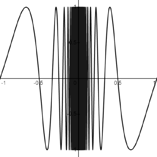
Figure \(\PageIndex{11}\): The graph of \(f(x)= \sin{\left( \pi/x \right)}\) shows a that the values of \(f\) varying wildly as \(x\) gets close to \(0\).

---

Time-Sensitive Advice: HawkConnect

What is HawkConnect?

In the past, navigating through all the student resources (EOPS, TRIO, MI CASA, etc.) required you to go to individual sites and apply individually for each program. HawkConnect now unifies the entire process into a single, guided application process.

To learn more about HawkConnect and to apply, go to the CRC Support Services website.

---

Success in Mathematics: Show Your Work

Many mathematics exams include the statement, "Show Your Work" (if it's not explicitly written, then it is implied). The exact meaning of these words can change from one professor to another; however, they usually mean that you need to show more than just the answer to a problem. You need to explain or show how you found the answer. Your responsibility is to learn what "Show Your Work" means to your instructor.

Why do you need to show your work?

Your authentic work (e.g., without use of A.I., tutors, or any other external help) demonstrates what you know. It shows what you understand and what you do not understand. By looking at your work and the work of others, an instructor can help you improve your understanding.

Everyone makes mistakes. To learn from these mistakes, you need to be able to find them. If you show your work, you can go back and find mistakes. This helps you identify misunderstandings and bad habits. Without your work, all you can do is start over.

Finally, although you may be able to do a problem "in your head," this will not always be possible. The problems get more challenging and involve more detail as we move forward. Showing your work now develops the habits and procedures you will need to do math in the future.

Here are some questions about this topic that may help you succeed in this class (and possibly many other classes as well):

1. A student did a homework exercise. She checked her answer with the back of the book. It was wrong. So, she erased her work and started over. Why should she not erase her work?
2. A student did a homework exercise. He checked his answer with the back of the book. It was wrong. He marked the problem on his homework with an asterisk. He went on with the assignment. He never went back to the problem. Why is it essential for this student to finish the problem?

If you are unsure about the answers to either of these questions, feel free to ask your instructor - that's what they are there for!