1.2.3: Additional Exercises

Last updated
Save as PDF

Page ID: 192219

$ \newcommand{\vecs}[1]{\overset { \scriptstyle \rightharpoonup} {\mathbf{#1}} } $

$ \newcommand{\vecd}[1]{\overset{-\!-\!\rightharpoonup}{\vphantom{a}\smash {#1}}} $

$ \newcommand{\dsum}{\displaystyle\sum\limits} $

$ \newcommand{\dint}{\displaystyle\int\limits} $

$ \newcommand{\dlim}{\displaystyle\lim\limits} $

$ \newcommand{\id}{\mathrm{id}}$ $ \newcommand{\Span}{\mathrm{span}}$

( \newcommand{\kernel}{\mathrm{null}\,}\) $ \newcommand{\range}{\mathrm{range}\,}$

$ \newcommand{\RealPart}{\mathrm{Re}}$ $ \newcommand{\ImaginaryPart}{\mathrm{Im}}$

$ \newcommand{\Argument}{\mathrm{Arg}}$ $ \newcommand{\norm}[1]{\| #1 \|}$

$ \newcommand{\inner}[2]{\langle #1, #2 \rangle}$

$ \newcommand{\Span}{\mathrm{span}}$

$ \newcommand{\id}{\mathrm{id}}$

$ \newcommand{\Span}{\mathrm{span}}$

$ \newcommand{\kernel}{\mathrm{null}\,}$

$ \newcommand{\range}{\mathrm{range}\,}$

$ \newcommand{\RealPart}{\mathrm{Re}}$

$ \newcommand{\ImaginaryPart}{\mathrm{Im}}$

$ \newcommand{\Argument}{\mathrm{Arg}}$

$ \newcommand{\norm}[1]{\| #1 \|}$

$ \newcommand{\inner}[2]{\langle #1, #2 \rangle}$

$ \newcommand{\Span}{\mathrm{span}}$ $ \newcommand{\AA}{\unicode[.8,0]{x212B}}$

$ \newcommand{\vectorA}[1]{\vec{#1}} % arrow$

$ \newcommand{\vectorAt}[1]{\vec{\text{#1}}} % arrow$

$ \newcommand{\vectorB}[1]{\overset { \scriptstyle \rightharpoonup} {\mathbf{#1}} } $

$ \newcommand{\vectorC}[1]{\textbf{#1}} $

$ \newcommand{\vectorD}[1]{\overrightarrow{#1}} $

$ \newcommand{\vectorDt}[1]{\overrightarrow{\text{#1}}} $

$ \newcommand{\vectE}[1]{\overset{-\!-\!\rightharpoonup}{\vphantom{a}\smash{\mathbf {#1}}}} $

$ \newcommand{\vecs}[1]{\overset { \scriptstyle \rightharpoonup} {\mathbf{#1}} } $

$\newcommand{\longvect}{\overrightarrow}$

$ \newcommand{\vecd}[1]{\overset{-\!-\!\rightharpoonup}{\vphantom{a}\smash {#1}}} $

$\newcommand{\ket}[1]{\left| #1 \right>}$
$\newcommand{\bra}[1]{\left< #1 \right|}$
$\newcommand{\braket}[2]{\left< #1 \vphantom{#2} \right| \left. #2 \vphantom{#1} \right>}$
$\newcommand{\braopket}[3]{\left< #1 \vphantom{#2}\vphantom{#3} \right| #2 \vphantom{#1}\vphantom{#3} \left| #3 \vphantom{#1}\vphantom{#2} \right>}$
$\newcommand{\qmvec}[1]{\mathbf{\vec{#1}}}$
$\newcommand{\op}[1]{\hat{\mathbf{#1}}}$
$\newcommand{\expect}[1]{\langle #1 \rangle}$
$\newcommand{\dfn}[1]{\emph{\textbf{#1}}}$

$\newcommand{\avec}{\mathbf a}$ $\newcommand{\bvec}{\mathbf b}$ $\newcommand{\cvec}{\mathbf c}$ $\newcommand{\dvec}{\mathbf d}$ $\newcommand{\dtil}{\widetilde{\mathbf d}}$ $\newcommand{\evec}{\mathbf e}$ $\newcommand{\fvec}{\mathbf f}$ $\newcommand{\nvec}{\mathbf n}$ $\newcommand{\pvec}{\mathbf p}$ $\newcommand{\qvec}{\mathbf q}$ $\newcommand{\svec}{\mathbf s}$ $\newcommand{\tvec}{\mathbf t}$ $\newcommand{\uvec}{\mathbf u}$ $\newcommand{\vvec}{\mathbf v}$ $\newcommand{\wvec}{\mathbf w}$ $\newcommand{\xvec}{\mathbf x}$ $\newcommand{\yvec}{\mathbf y}$ $\newcommand{\zvec}{\mathbf z}$ $\newcommand{\rvec}{\mathbf r}$ $\newcommand{\mvec}{\mathbf m}$ $\newcommand{\zerovec}{\mathbf 0}$ $\newcommand{\onevec}{\mathbf 1}$ $\newcommand{\real}{\mathbb R}$ $\newcommand{\twovec}[2]{\left[\begin{array}{r}#1 \\ #2 \end{array}\right]}$ $\newcommand{\ctwovec}[2]{\left[\begin{array}{c}#1 \\ #2 \end{array}\right]}$ $\newcommand{\threevec}[3]{\left[\begin{array}{r}#1 \\ #2 \\ #3 \end{array}\right]}$ $\newcommand{\cthreevec}[3]{\left[\begin{array}{c}#1 \\ #2 \\ #3 \end{array}\right]}$ $\newcommand{\fourvec}[4]{\left[\begin{array}{r}#1 \\ #2 \\ #3 \\ #4 \end{array}\right]}$ $\newcommand{\cfourvec}[4]{\left[\begin{array}{c}#1 \\ #2 \\ #3 \\ #4 \end{array}\right]}$ $\newcommand{\fivevec}[5]{\left[\begin{array}{r}#1 \\ #2 \\ #3 \\ #4 \\ #5 \\ \end{array}\right]}$ $\newcommand{\cfivevec}[5]{\left[\begin{array}{c}#1 \\ #2 \\ #3 \\ #4 \\ #5 \\ \end{array}\right]}$ $\newcommand{\mattwo}[4]{\left[\begin{array}{rr}#1 \amp #2 \\ #3 \amp #4 \\ \end{array}\right]}$ $\newcommand{\laspan}[1]{\text{Span}\{#1\}}$ $\newcommand{\bcal}{\cal B}$ $\newcommand{\ccal}{\cal C}$ $\newcommand{\scal}{\cal S}$ $\newcommand{\wcal}{\cal W}$ $\newcommand{\ecal}{\cal E}$ $\newcommand{\coords}[2]{\left\{#1\right\}_{#2}}$ $\newcommand{\gray}[1]{\color{gray}{#1}}$ $\newcommand{\lgray}[1]{\color{lightgray}{#1}}$ $\newcommand{\rank}{\operatorname{rank}}$ $\newcommand{\row}{\text{Row}}$ $\newcommand{\col}{\text{Col}}$ $\renewcommand{\row}{\text{Row}}$ $\newcommand{\nul}{\text{Nul}}$ $\newcommand{\var}{\text{Var}}$ $\newcommand{\corr}{\text{corr}}$ $\newcommand{\len}[1]{\left|#1\right|}$ $\newcommand{\bbar}{\overline{\bvec}}$ $\newcommand{\bhat}{\widehat{\bvec}}$ $\newcommand{\bperp}{\bvec^\perp}$ $\newcommand{\xhat}{\widehat{\xvec}}$ $\newcommand{\vhat}{\widehat{\vvec}}$ $\newcommand{\uhat}{\widehat{\uvec}}$ $\newcommand{\what}{\widehat{\wvec}}$ $\newcommand{\Sighat}{\widehat{\Sigma}}$ $\newcommand{\lt}{<}$ $\newcommand{\gt}{>}$ $\newcommand{\amp}{&}$ $\definecolor{fillinmathshade}{gray}{0.9}$

Reading Questions

How does using a graph help in estimating $ \displaystyle \lim_{x \to a} f(x)$?
What are two potential pitfalls when trying to determine a limit solely from a graph?
If a graph of $f(x)$ has an open circle at the point $(a, L)$ but the curve smoothly approaches this point from both the left and the right, what is $ \displaystyle \lim_{x \to a} f(x)$? What can be said about $f(a)$?
Explain how to find $ \displaystyle \lim_{x \to a^-} f(x)$ and $ \displaystyle \lim_{x \to a^+} f(x)$ by looking at a graph.
If $ \displaystyle \lim_{x \to a^-} f(x) = L_1$ and $ \displaystyle \lim_{x \to a^+} f(x) = L_2$, where $L_1 \neq L_2$, what can you conclude about $ \displaystyle \lim_{x \to a} f(x)$ based on its graph?
What does the graph of a function typically show near a value $x=a$ if $ \displaystyle \lim_{x \to a} f(x) = \infty$?
According to the definition provided in this section, what conditions involving limits must be met for a function $f(x)$ to have a vertical asymptote at $x=a$?
When evaluating a limit like $ \displaystyle \lim_{x \to a} \frac{N(x)}{D(x)}$ where $N(x) \to k \neq 0$ and $D(x) \to 0$, what information about $N(x)$ and $D(x)$ as $x \to a$ is needed to determine if the limit is $\infty$ or $-\infty$?
Why is it incorrect to write $ \displaystyle \lim_{x \to c} f(x) = \frac{k}{0}$? What notation should be used to show the conceptual steps?
In Example 7, part d, $ \displaystyle \lim_{x \to (\pi/2)^-} \ln(\cot x)$, describe the step-by-step thought process for evaluating this limit conceptually by considering the behavior of the inner function $\cot x$ and then the outer function $\ln(u)$.
How does Figure 6 (the graph of $f(x) = \sin(1/x)$) visually demonstrate that $ \displaystyle \lim_{x \to 0} \sin(1/x)$ does not exist?
What does the graph in Figure 10 illustrate about the relationship between $f(c)$ and $ \displaystyle \lim_{x \to c} f(x)$ at various points $c$?

Homework

In exercises 1 - 2, set up a table of values and round to eight significant digits. Based on the table of values, make a guess about what the limit is. Then, use a calculator to graph the function and determine the limit. Was the conjecture correct? If not, why does the method of tables fail?

1) $\displaystyle \lim_{ \theta \to 0}\sin\left(\frac{ \pi }{ \theta }\right)$

$ \theta $	$\sin\left(\frac{ \pi }{ \theta }\right)$	$ \theta $	$\sin\left(\frac{ \pi }{ \theta }\right)$
-0.1	a.	0.1	e.
-0.01	b.	0.01	f.
-0.001	c.	0.001	g.
-0.0001	d.	0.0001	h.

2) $\displaystyle \lim_{ \alpha \to 0^+} \frac{1}{ \alpha }\cos\left(\frac{ \pi }{ \alpha }\right)$

$\alpha$	$\frac{1}{ \alpha }\cos\left(\frac{ \pi }{ \alpha }\right)$
0.1	a.
0.01	b.
0.001	c.
0.0001	d.

In exercises 3 - 6, consider the graph of the function$y=f(x)$ shown here. Which of the statements about $y=f(x)$ are true and which are false? Explain why a statement is false.

$A graph of a piecewise function with three segments and a point. The first segment is a curve opening upward with vertex at (-8, -6). This vertex is an open circle, and there is a closed circle instead at (-8, -3). The segment ends at (-2,3), where there is a closed circle. The second segment stretches up asymptotically to infinity along x=-2, changes direction to increasing at about (0,1.25), increases until about (2.25, 3), and decreases until (6,2), where there is an open circle. The last segment starts at (6,5), increases slightly, and then decreases into quadrant four, crossing the x axis at (10,0). All of the changes in direction are smooth curves.$

3) $\displaystyle \lim_{x \to 10}f(x)=0$

4) $\displaystyle \lim_{x \to −2^+}f(x)=3$

5) $\displaystyle \lim_{x \to −8}f(x)=f(−8)$

6) $\displaystyle \lim_{x \to 6}f(x)=5$

In exercises 7 - 11, use the following graph of the function $y=f(x)$ to find the values, if possible. Estimate when necessary.

$A graph of a piecewise function with two segments. The first segment exists for x <=1, and the second segment exists for x > 1. The first segment is linear with a slope of 1 and goes through the origin. Its endpoint is a closed circle at (1,1). The second segment is also linear with a slope of -1. It begins with the open circle at (1,2).$

7) $\displaystyle \lim_{x \to 1^−}f(x)$

8) $\displaystyle \lim_{x \to 1^+}f(x)$

9) $\displaystyle \lim_{x \to 1}f(x)$

10) $\displaystyle \lim_{x \to 2}f(x)$

11) $f(1)$

In exercises 12 - 15, use the graph of the function $y=f(x)$ shown here to find the values, if possible. Estimate when necessary.

$A graph of a piecewise function with two segments. The first is a linear function for x < 0. There is an open circle at (0,1), and its slope is -1. The second segment is the right half of a parabola opening upward. Its vertex is a closed circle at (0, -4), and it goes through the point (2,0).$

12) $\displaystyle \lim_{x \to 0^−}f(x)$

13) $\displaystyle \lim_{x \to 0^+}f(x)$

14) $\displaystyle \lim_{x \to 0}f(x)$

15) $\displaystyle \lim_{x \to 2}f(x)$

In exercises 16 - 21, use the graph of the function $y=f(x)$ shown here to find the values, if possible. Estimate when necessary.

$A graph of a piecewise function with three segments, all linear. The first exists for x < -2, has a slope of 1, and ends at the open circle at (-2, 0). The second exists over the interval [-2, 2], has a slope of -1, goes through the origin, and has closed circles at its endpoints (-2, 2) and (2,-2). The third exists for x>2, has a slope of 1, and begins at the open circle (2,2).$

16) $\displaystyle \lim_{x \to −2^−}f(x)$

17) $\displaystyle \lim_{x \to −2^+}f(x)$

18) $\displaystyle \lim_{x \to −2}f(x)$

19) $\displaystyle \lim_{x \to 2^−}f(x)$

20) $\displaystyle \lim_{x \to 2^+}f(x)$

21) $\displaystyle \lim_{x \to 2}f(x)$

In exercises 22 - 24, use the graph of the function $y=g(x)$ shown here to find the values, if possible. Estimate when necessary.

$A graph of a piecewise function with two segments. The first exists for x>=0 and is the left half of an upward opening parabola with vertex at the closed circle (0,3). The second exists for x>0 and is the right half of a downward opening parabola with vertex at the open circle (0,0).$

22) $\displaystyle \lim_{x \to 0^−}g(x)$

23) $\displaystyle \lim_{x \to 0^+}g(x)$

24) $\displaystyle \lim_{x \to 0}g(x)$

In exercises 25 - 27, use the graph of the function $y=h(x)$ shown here to find the values, if possible. Estimate when necessary.

$A graph of a function with two curves approaching 0 from quadrant 1 and quadrant 3. The curve in quadrant one appears to be the top half of a parabola opening to the right of the y axis along the x axis with vertex at the origin. The curve in quadrant three appears to be the left half of a parabola opening downward with vertex at the origin.$

25) $\displaystyle \lim_{x \to 0^−}h(x)$

26) $\displaystyle \lim_{x \to 0^+}h(x)$

27) $\displaystyle \lim_{x \to 0}h(x)$

In exercises 28 - 32, use the graph of the function $y=f(x)$ shown here to find the values, if possible. Estimate when necessary.

$A graph with a curve and a point. The point is a closed circle at (0,-2). The curve is part of an upward opening parabola with vertex at (1,-1). It exists for x > 0, and there is a closed circle at the origin.$

28) $\displaystyle \lim_{x \to 0^−}f(x)$

29) $\displaystyle \lim_{x \to 0^+}f(x)$

30) $\displaystyle \lim_{x \to 0}f(x)$

31) $\displaystyle \lim_{x \to 1}f(x)$

32) $\displaystyle \lim_{x \to 2}f(x)$

In exercises 33 - 37, sketch the graph of a function with the given properties.

33) \[ \lim_{x \to 2}f(x)=1, \nonumber \]\[ \lim_{x \to 4^−}f(x)=3, \nonumber \]\[\lim_{x \to 4^+}f(x)=6, \nonumber \]\[ \text{ and } x=4 \text{ is not defined.}\nonumber \]

34) \[ \lim_{x \to − \infty }f(x)=0, \nonumber \]\[ \lim_{x \to −1^−}f(x)=− \infty , \nonumber \]\[ \lim_{x \to −1^+}f(x)= \infty , \nonumber \]\[ \lim_{x \to 0}f(x)=f(0), \nonumber \]\[ f(0)=1, \nonumber \]\[ \text{ and } \lim_{x \to \infty }f(x)=− \infty. \nonumber \]

35) \[ \lim_{x \to − \infty }f(x)=2, \nonumber \]\[ \lim_{x \to 3^−}f(x)=− \infty , \nonumber \]\[ \lim_{x \to 3^+}f(x)= \infty , \nonumber \]\[ \lim_{x \to \infty }f(x)=2,\nonumber \]\[\text{ and } f(0)=-\dfrac{1}{3}. \nonumber \]

36) \[ \lim_{x \to − \infty }f(x)=2, \nonumber \]\[ \lim_{x \to −2}f(x)=− \infty , \nonumber \]\[ \lim_{x \to \infty }f(x)=2, \nonumber \]\[ \text{ and } f(0)=0. \nonumber \]

37) \[ \lim_{x \to − \infty }f(x)=0, \nonumber \]\[\lim_{x \to −1^−}f(x)= \infty , \nonumber \]\[ \lim_{x \to −1^+}f(x)=− \infty , \nonumber \]\[ f(0)=−1, \nonumber \]\[ \lim_{x \to 1^−}f(x)=− \infty , \nonumber \]\[ \lim_{x \to 1^+}f(x)= \infty , \nonumber \]\[ \text{ and } \lim_{x \to \infty }f(x)=0. \nonumber \]

38) Shock waves arise in many physical applications, ranging from supernovas to detonation waves. A graph of the density of a shock wave with respect to distance, $x$, is shown here. We are mainly interested in the location of the front of the shock, labeled $X_{SF}$ in the diagram.

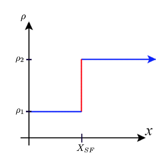
$A graph in quadrant one of the density of a shockwave with three labeled points: p1 and p2 on the y axis, with p1 > p2, and xsf on the x axis. It consists of y= p1 from 0 to xsf, x = xsf from y= p1 to y=p2, and y=p2 for values greater than or equal to xsf.$

a. Evaluate $\displaystyle \lim_{x \to X_{SF}^+} \rho (x)$.

b. Evaluate $\displaystyle \lim_{x \to X_{SF}^−} \rho (x)$.

c. Evaluate $\displaystyle \lim_{x \to X_{SF}} \rho (x)$. Explain the physical meanings behind your answers.

Search

Text Color

Text Size

Margin Size

Font Type