1.7: The Precise Definitions of Limits Involving Infinity

Section Preview

Note to the Instructor (click to expand)

This section rounds out the precise definition of a limit by presenting the definitions involving infinities. As with the previous section, this material is NOT optional.

Core Prerequisites (i.e., "Understanding the Lesson"): The following prerequisite topics (which have not already been listed as prerequisites in previous sections of this text) are required to understand the core concepts in this lesson.

(click to expand)

• Logarithmic Functions
  • The Basics of Logarithmic Functions

Operational Prerequisites (i.e., "Completing the Homework"): The following prerequisite topics (which have not already been listed as prerequisites in previous sections of this text) are needed to complete the homework.

(click to expand)

• Arithmetic
  • Mathematical Operations — Higher-Index Roots
• Simplifying Expressions
  • Laws of Exponents — Zero and Negative Exponent Rules
  • Simplifying Expressions Involving Positive Rational Exponents
• Solving Equations
  • Solving Exponential Equations
  • Solving Logarithmic Equations

The following is a list of learning objectives for this section.

Learning Objectives (click to expand)

• Describe the precise definition of a limit for infinite limits, at finite points and infinity.
• Prove finite and infinite limits using the precise definition of a limit.

The previous section walked us slowly through the theory of finite limits at finite numbers. Instead of evaluating limits, we proved limits using \(\epsilon-\delta\) proofs. We now turn our attention to limits involving infinity. There are three such limits:

1. infinite limits at finite numbers,
2. finite limits at infinity, and
3. infinite limits at infinity.

We treat each of these separately and pull all limit proof styles into a unified theory at the end of the section.

Infinite Limits at Finite Numbers

Previously, we learned how to conceptually investigate limits of the form \[\displaystyle \lim_{x \to 1}{\dfrac{1}{(x - 1)^2}}.\nonumber\] These types of limits are called infinite limits at finite numbers because their limits approach infinity as \(x\) approaches a finite number.

To investigate this limit, we stated that \((x - 1)^2 \to 0^+\) as \(x \to 1\). Thus, \(\frac{1}{(x - 1)^2} \to \frac{1}{0^+} \to \infty\).

At the time, these arguments were sufficient, if not precise; however, we now turn our attention to proving \[\displaystyle \lim_{x \to 1}{\dfrac{1}{(x - 1)^2}} = \infty. \label{ifex}\] To understand the structure of the proof for infinite limits at finite numbers, we need to discuss the structure of the traditional \(\epsilon-\delta\) proof.

Given \(\displaystyle \lim_{x \to a}{(f(x))} = L\), where \(a\) and \(L\) are finite, it should now make sense that we require an \(\epsilon\)-neighborhood about the finite number \(L\), and a \(\delta\)-neighborhood about the finite number \(a\); however, in the limit \(\ref{ifex}\), \(L = \infty\) is not finite. Therefore, creating a small \(\epsilon\)-neighborhood about \(L\) makes no sense. We cannot bound \(\infty\) in a small \(\epsilon\)-neighborhood. Thus, our precise definition needs some adjustment for this type of limit.

Figure \(\PageIndex{1}\) shows the graph of \(f(x) = \frac{1}{(x - 1)^2}\).

Figure \(\PageIndex{1}\): \(f(x) = \frac{1}{(x - 1)^2}\)

While it's easy to see that the function values, \(f(x)\), tend to \(\infty\) as our \(\delta\)-neighborhood centered at \(x = 1\) gets smaller and smaller, this is not a proof. What we need is for someone to challenge us (as they did with the \(\epsilon\)-gauntlet in the previous section) and say, "I bet you cannot find a small enough \(\delta\)-neighborhood centered at \(x = 1\) so that all the corresponding function values are above... oh, let's say a billion!" And this is the key to the structure of the precise definition of an infinite limit at a finite point. Instead of "for any given \(\epsilon \gt 0\)," we are faced with "for any given \(N \ggg 0\)," where the notation \(\ggg\) means "much greater than." And instead of a small \(\epsilon\)-neighborhood around \(L\), we are challenged with getting the function values above (or below, if the limit is tending to \(-\infty\)) some massively large number \(N\). Visually, it looks a bit like Figure \(\PageIndex{2}\).

Figure \(\PageIndex{2}\)

We can now formalize the precise definition of an infinite limit at a finite number.

Definition: Infinite Limit at a Finite Number (Precise Definition)

Let \(f(x)\) be defined for all \(x \neq a\) over an open interval containing \(a\). Then we say \[\lim_{x \to a}{f(x)} = \infty\nonumber\] if for every \(N \ggg 0\), there exists a \(\delta \gt 0\), such that if \(0 \lt |x-a| \lt \delta\), then \(f(x) \gt N\).

Stated with symbolic logic, \[\lim_{x \to a}{f(x)} = \infty\nonumber\] means \[\forall N \ggg 0, \quad \exists \delta \gt 0 \ni\nonumber\] \[0 \lt |x - a| \lt \delta \implies f(x) \gt N.\nonumber\] Additionally, we say \[\lim_{x \to a}{f(x)} = -\infty\nonumber\] if for every \(N \lll 0\), there exists a \(\delta \gt 0\), such that if \(0 \lt |x-a| \lt \delta\), then \(f(x) \lt N\).

Stated with symbolic logic, \[\lim_{x \to a}{f(x)} = -\infty\nonumber\] means \[\forall N \lll 0, \quad \exists \delta \gt 0 \ni\nonumber\] \[0 \lt |x - a| \lt \delta \implies f(x) \lt N.\nonumber\]

Let's see this in an example.

Example \(\PageIndex{1}\)

Prove \[\displaystyle \lim_{x \to 1}{\frac{1}{(x - 1)^2}} = \infty.\nonumber\]

Solution

PROOF For \(N \ggg 0\), let \(\delta = \frac{1}{\sqrt{N}}\). If \(0 \lt |x - 1| \lt \delta\), then \[\begin{array}{crcl} & |x - 1| & \lt & \dfrac{1}{\sqrt{N}} \\[16pt] \implies & (x - 1)^2 & \lt & \dfrac{1}{N} \\[16pt] \implies & \dfrac{1}{(x - 1)^2} & \gt & N \\[16pt] \implies & f(x) & \gt & N \\ \end{array}\nonumber\] Thus, we have proved the limit \[\displaystyle \lim_{x \to 1}{\dfrac{1}{(x - 1)^2}} = \infty.\nonumber\]

SCRATCH WORK We want to arrive at \[\dfrac{1}{(x - 1)^2} \gt N \quad \left( \text{consequent} \right)\nonumber\] given that \[0 \lt |x - 1| \lt \delta. \quad \left( \text{antecedent} \right)\nonumber\] Working backward from the consequent and trying to arrive at the antecedent, we get \[\begin{array}{rcl} \dfrac{1}{(x - 1)^2} \gt N & \implies & (x - 1)^2 \lt \dfrac{1}{N} \\[16pt] & \implies & |x - 1| \lt \dfrac{1}{\sqrt{N}} \\[16pt] & \implies & \text{Let }\delta = \dfrac{1}{\sqrt{N}} \\ \end{array}\nonumber\]

Interactive Element: The \(N–\delta\) Challenge — Infinite Limit at a Finite Number

The following Interactive Element might help you visualize how the \(\delta\)-neighborhood responds when the challenge value \(N\) grows.

Interact: Drag the red point up and down to change the challenge height \(N\).

Observation: No matter how high you push \(N\), the shaded \(\delta\)-neighborhood around \(x=1\) simply narrows, and inside it the curve still rises above \(y=N\). A valid \(\delta\) always exists, which is exactly what \(\lim_{x\to 1} f(x)=\infty\) means.

A few tripping points commonly arise while working with this material. It's important to remember the following from your prerequisite courses:

1. An inequality switches directions if you multiply or divide by a negative.
2. Applying an even power to an expression results in a positive value (this can be seen between the first and second steps of the proof in Example \(\PageIndex{1}\)).
3. \(\sqrt{\left( \blacksquare \right)^2} = \left| \blacksquare \right|\). This fact is used in the second-to-last step of the Scratch Work.

We will add to this list as we move forward, but if you have solid prerequisites, you have nothing to worry about.

Vertical Asymptotes

You have encountered vertical asymptotes in your algebra courses as part of the rational and logarithmic functions material. Moreover, you worked with them in Trigonometry. We now formalize their definition using Calculus.

Definition: Vertical Asymptote

The vertical line \(x = a\) is called a vertical asymptote of the function \(f(x)\) if at least one of the following is true: \[\begin{array}{ccccc} \displaystyle \lim_{x \to a}{f(x)} = \infty & \quad & \displaystyle \lim_{x \to a^-}{f(x)} = \infty & \quad & \displaystyle \lim_{x \to a^+}{f(x)} = \infty \\ \displaystyle \lim_{x \to a}{f(x)} = -\infty & \quad & \displaystyle \lim_{x \to a^-}{f(x)} = -\infty & \quad & \displaystyle \lim_{x \to a^+}{f(x)} = -\infty \\ \end{array}\nonumber\]

Example \(\PageIndex{2}\)

Prove that \(x = -2\) is a vertical asymptote of \(f(x) = \ln{(x + 2)}.\)

Solution

From algebra, we know the domain of \(f(x) = \ln{(x + 2)}\) is \((-2 , \infty)\). Therefore, to prove \(x = -2\) is a vertical asymptote, we only need to concern ourselves with the one-sided limit \[\displaystyle \lim_{x \to -2^+}{\ln{(x + 2)}}.\nonumber\] We know that the graph of \(\ln{(x + 2)}\) tends to \(-\infty\) as \(x\) approaches \(-2\). Now we are asked to prove it. That is, we want to prove \[\displaystyle \lim_{x \to -2^+}{\ln{(x + 2)}} = -\infty.\nonumber\]

PROOF For \(N \lll 0\), let \(\delta = e^N\). If \(0 \lt x - (-2) \lt \delta\), then \[\begin{array}{crcl} & x + 2 & \lt & e^N \\ \implies & \ln{(x + 2)} & \lt & N \\ \implies & f(x) & \lt & N \\ \end{array}\nonumber\] Thus, we have proved the limit \[\displaystyle \lim_{x \to -2}{\ln{(x + 2)}} = -\infty.\nonumber\] Therefore, \(x = -2\) is a vertical asymptote of \(f(x) = \ln{(x + 2)}.\)

SCRATCH WORK We want to arrive at \[\ln{(x + 2)} \lt N \quad \left( \text{consequent} \right)\nonumber\] given that \[0 \lt x - (-2) = x + 2 \lt \delta. \quad \left( \text{antecedent} \right)\nonumber\] (Since \(x \to -2^+\), \(x \gt -2 \implies x + 2 \gt 0\).) Working backward from the consequent and trying to arrive at the antecedent, we get \[\begin{array}{rcl} \ln{(x + 2)} \lt N & \implies & x + 2 \lt e^N \\ & \implies & \text{Let }\delta = e^N \\ \end{array}\nonumber\]

Adding to that list of tripping points:

4. If \(x \lt y\), then \(e^x \lt e^y\) (this is a direct result of the fact that \(y = e^x\) is an increasing function). This allows us to rewrite inequalities like \(\ln{(x + 2)} \lt N\) as \(e^{\ln{(x + 2)}} \lt e^N \implies x + 2 \lt e^N\).
5. Stating that \(\delta = e^N\) might seem wrong to you because \(\delta\) is typically very small; however, pay close attention to the value of \(N\). In Example \(\PageIndex{2}\), \(N \lll 0\). Therefore, \(e^N\) is very small.

Finite Limits at Infinity

Consider \[\displaystyle \lim_{x \to \infty}{\dfrac{e^x - e^{-x}}{e^x + e^{-x}}}.\nonumber\] Some algebraic manipulation is necessary to see how this limit behaves. \[\begin{array}{rclcl} \displaystyle \lim_{x \to \infty}{\dfrac{e^x - e^{-x}}{e^x + e^{-x}}} & = & \displaystyle \lim_{x \to \infty}{\dfrac{1 - e^{-2x}}{1 + e^{-2x}}} & \quad & \left( \text{multiplying by }\dfrac{1/e^x}{1/e^x} \right) \\[16pt] & = & \displaystyle \lim_{x \to \infty}{\dfrac{1 - \frac{1}{e^{2x}}}{1 + \frac{1}{e^{2x}}}} & & \\[16pt] & = & \dfrac{1 - 0}{1 + 0} & \quad & \left( \dfrac{1}{e^{2x}} \to 0 \text{ as } x \to \infty \right) \\[16pt] & = & 1 & \\ \end{array}\nonumber\] The second-to-last step in this derivation relied on assumptions that \(\frac{1}{e^{2x}} \to 0\) as \(x \to \infty\). In previous sections, we bolstered this assumption with a "hand-waving" argument, saying, "Well, it's obvious that the denominator of \(\frac{1}{e^{2x}}\) goes to infinity as \(x\) goes to infinity. Therefore, \(1\) over something going to infinity will shrink to \(0\)." However, this is not a rigorous mathematical justification.

So, how can we prove \[\displaystyle \lim_{x \to \infty}{\dfrac{1}{e^{kx}}} = 0 \text{ }\left( \text{for }k \gt 0 \right), \label{fiex1}\] which in turn will prove \[\displaystyle \lim_{x \to \infty}{\dfrac{e^x - e^{-x}}{e^x + e^{-x}}} = 1? \label{fiex2}\] Limits like \(\ref{fiex1}\) and \(\ref{fiex2}\) are called finite limits at infinity because the limits become finite (\(0\) in \(\ref{fiex1}\) and \(1\) in \(\ref{fiex2}\)) as \(x\) approaches infinity.

To understand the proof structure for finite limits at infinity, we again need to modify the traditional \(\epsilon-\delta\) proof. In \(\ref{fiex1}\), \(L = 0\) is finite, but \(a = \infty\) is not finite. Therefore, creating a small \(\delta\)-neighborhood about \(a\) makes no sense. Just as before, we cannot bound \(\infty\) in a small \(\delta\)-neighborhood.

Figure \(\PageIndex{3}\) shows the graph of \(f(x) = \frac{1}{e^{2x}}\) (we will worry about \(\frac{1}{e^{kx}}\) later).

Figure \(\PageIndex{3}\): \(f(x) = \frac{1}{e^{2x}}\)

If the claim is that \[\displaystyle \lim_{x \to \infty}{\dfrac{1}{e^{2x}}} = 0,\nonumber\] then someone is going to throw the \(\epsilon\)-gauntlet to challenge us to force the function to be bounded within the interval \((0-\epsilon,0+\epsilon)\), as in Figure \(\PageIndex{4}\).

Figure \(\PageIndex{4}\)

It's apparent from Figure \(\PageIndex{4}\) that, as long as \(x\) is large enough, \(-\epsilon \lt f(x) \lt \epsilon\). In fact, we see in Figure \(\PageIndex{5}\), as long as \(x \gt M\), \(|f(x) - 0| \lt \epsilon\).

Figure \(\PageIndex{5}\)

This gives us great insight into the formal definition of finite limits at infinity.

Definition: Finite Limit at Infinity (Precise Definition)

Let \(f(x)\) be defined for all \(x \gt a\). Then we say \[\lim_{x \to \infty}{f(x)} = L\nonumber\] if for every \(\epsilon \gt 0\), there exists a number \(M \gt 0\), such that if \(x \gt M\), then \(|f(x) - L| \lt \epsilon\).

Stated with symbolic logic, \[\lim_{x \to \infty}{f(x)} = L\nonumber\] means \[\forall \epsilon \gt 0, \quad \exists M \gt 0 \ni\nonumber\] \[x \gt M \implies |f(x) - L| \lt \epsilon.\nonumber\] Additionally, we say \[\lim_{x \to -\infty}{f(x)} = L\nonumber\] if for every \(\epsilon \gt 0\), there exists a number \(M \lt 0\), such that if \(x \lt M\), then \(|f(x) - L| \lt \epsilon\).

Stated with symbolic logic, \[\lim_{x \to -\infty}{f(x)} = L\nonumber\] means \[\forall \epsilon \gt 0, \quad \exists M \lt 0 \ni\nonumber\] \[x \lt M \implies |f(x) - L| \lt \epsilon.\nonumber\]

Interactive Element: The \(\epsilon–M\) Challenge — Finite Limit at Infinity

The following Interactive Element might help you visualize how the threshold \(M\) responds as the \(\varepsilon\)-band tightens around the horizontal asymptote \(y=0\).

Interact: Drag the red point down to shrink the \(\varepsilon\)-band around \(y=0\).

Observation: As the band narrows, the threshold \(x=M\) slides right, but past it the curve is always trapped inside the band. A valid \(M\) always exists, so \(\lim_{x\to\infty} e^{-2x}=0\).

We now introduce two very powerful theorems. The proofs of each of these theorems showcase how to use the precise definition of a finite limit at infinity.

Theorem

\[\displaystyle \lim_{x \to \infty}{e^{-x}} = 0\nonumber\]

Proof

PROOF For \(\epsilon \gt 0\), let \(M = -\ln{(\epsilon)}\). If \(x \gt M\), then \[\begin{array}{crcl} & x & \gt & -\ln{(\epsilon)} \\ \implies & -x & \lt & \ln{(\epsilon)} \\ \implies & e^{-x} & \lt & \epsilon \\ \implies & \left|e^{-x} - 0\right| & \lt & \epsilon \\ \implies & \left|f(x) - L\right| & \lt & \epsilon \\ \end{array}\nonumber\] Thus, we have proved the limit \[\displaystyle \lim_{x \to \infty}{e^{-x}} = 0.\nonumber\]

SCRATCH WORK We want to arrive at \[|e^{-x} - 0| \lt \epsilon \quad \left( \text{consequent} \right)\nonumber\] given that \[x \gt M. \quad \left( \text{antecedent} \right)\nonumber\] (Since \(x \to \infty\), \(x \gt M\).) Working backward from the consequent and trying to arrive at the antecedent, we get \[\begin{array}{rcl} |e^{-x} - 0| \lt \epsilon & \implies & e^{-x} \lt \epsilon \\ & \implies & -x \lt \ln{(\epsilon)} \\ & \implies & x \gt -\ln{(\epsilon)} \\ & \implies & \text{Let }M = -\ln{(\epsilon)} \\ \end{array}\nonumber\]

Again, adding to our list of tripping points:

6. \(|e^{-x}| = e^{-x}\) because \(e^{-x} \gt 0\).
7. In the proof of Theorem \(\PageIndex{1}\), we found \(M = -\ln{(\epsilon)}\); however, we also stated that \(M \gt 0\). How can this be?
   Don't be fooled into thinking an "opposite sign" (\(-\)) means that you're dealing with a negative number. In reality, \(\epsilon\) is a very small positive number. Therefore, \(\ln{(\epsilon)}\) is negative. Hence, \(M = -\ln{(\epsilon)}\) is positive.

The previous theorem begets a simple corollary.

Corollary

If \(k \gt 0\), \[\displaystyle \lim_{x \to \infty}{e^{-kx}} = 0\nonumber\]

Proof

\[\begin{array}{rclcl} \displaystyle \lim_{x \to \infty}{e^{-kx}} & = & \displaystyle \lim_{x \to \infty}{\left(e^{-x}\right)^k} & & \\ & = & \left(\displaystyle \lim_{x \to \infty}{e^{-x}}\right)^k & \quad & \left( \text{Power Law of Limits} \right) \\ & = & \left(0\right)^k & & \\ & = & 0 & \\ \end{array}\nonumber\]

The following theorem will be used throughout Calculus.

Theorem

If \(p \gt 0\) is a rational number, then \[\displaystyle \lim_{x \to \infty}{\dfrac{1}{x^p}} = 0.\nonumber\] If \(p \gt 0\) is a rational number such that \(x^p\) is defined for all \(x\), then \[\displaystyle \lim_{x \to -\infty}{\dfrac{1}{x^p}} = 0.\nonumber\]

Proof

PROOF (for \(\displaystyle \lim_{x \to \infty}{\frac{1}{x^p}} = 0\)) For \(\epsilon \gt 0\), let \(M = \frac{1}{\epsilon^{1/p}}\). If \(x \gt M\), then \[\begin{array}{crcl} & x & \gt & \dfrac{1}{\epsilon^{1/p}} \\[16pt] \implies & x^p & \gt & \dfrac{1}{\epsilon} \\[16pt] \implies & \dfrac{1}{x^p} & \lt & \epsilon \\[16pt] \implies & \left|\dfrac{1}{x^p} - 0\right| & \lt & \epsilon \\[16pt] \implies & \left|f(x) - L\right| & \lt & \epsilon \\ \end{array}\nonumber\] Thus, we have proved the limit \[\displaystyle \lim_{x \to \infty}{\dfrac{1}{x^p}} = 0.\nonumber\]

SCRATCH WORK (for \(\displaystyle \lim_{x \to \infty}{\frac{1}{x^p}} = 0\)) We want to arrive at \[\left|\dfrac{1}{x^p} - 0\right| \lt \epsilon \quad \left( \text{consequent} \right)\nonumber\] given that \[x \gt M. \quad \left( \text{antecedent} \right)\nonumber\] Working backward from the consequent, and trying to arrive at the antecedent, we get \[\begin{array}{rcl} \left|\dfrac{1}{x^p} - 0\right| \lt \epsilon & \implies & \dfrac{1}{x^p} \lt \epsilon \\[16pt] & \implies & x^p \gt \dfrac{1}{\epsilon} \\[16pt] & \implies & x \gt \dfrac{1}{\epsilon^{1/p}} \\[16pt] & \implies & \text{Let }M = \dfrac{1}{\epsilon^{1/p}} \\ \end{array}\nonumber\]

The proof of the second half of this theorem is left as a homework exercise.

As before, the proof of this theorem adds to our list of tripping points.

8. If \(x \gt 0\), then \(\left| \frac{1}{x^p} - 0 \right| = \frac{1}{x^p}\).

Horizontal Asymptotes

We have already introduced the definition of a horizontal asymptote; however, we repeat it here due to the connection with the finite limit at infinity.

Definition: Horizontal Asymptote

The vertical line \(y = L\) is called a horizontal asymptote of the function \(f(x)\) if at least one of the following is true: \[\begin{array}{ccccc} \displaystyle \lim_{x \to \infty}{f(x)} = L & \quad & \text{ or } & \quad & \displaystyle \lim_{x \to -\infty}{f(x)} = L \\ \end{array}\nonumber\]

Infinite Limits at Infinity

Up to this point, we have allowed ourselves the luxury of assuming \[\displaystyle \lim_{x \to \infty}{3^x} = \infty; \label{iiex1}\] however, it is at this moment that we need to prove this assumption is true. Limits of the form \(\ref{iiex1}\) are called infinite limits at infinity because the function tends to infinity (or negative infinity) and \(x\) tends to infinity (or negative infinity).

As with all our work in this section, developing the precise definition of an infinite limit at infinity requires adjusting the traditional \(\epsilon-\delta\) definition of a limit.

Since both \(x\) and the function are approaching infinity in \(\ref{iiex1}\), it is impossible for us to say, "For any given \(\epsilon \gt 0\), there exists a \(\delta \gt 0\)," because there is no way for us to contain infinity in a small interval (whether an \(\epsilon\)- or \(\delta\)-neighborhood).

So, how do we adjust the definition? Consider the following figure.

Figure \(\PageIndex{6}\): \(f(x) = 3^x\)

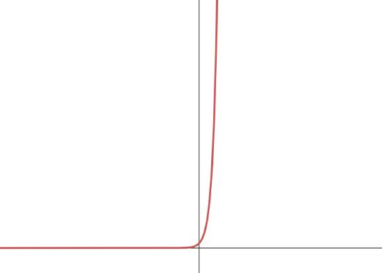
Instead of someone challenging us by throwing down an \(\epsilon\)-gauntlet, they are going to challenge us to get our function values above a colossal number (see Figure \(\PageIndex{7}\).

Figure \(\PageIndex{7}\)

That is, someone is going to hand us \(N \ggg 0\). Our job is to somehow find \(x\)-values whose function values are above the line \(y = N\). Figure \(\PageIndex{8}\) shows graphically how this is done.

Figure \(\PageIndex{8}\)

Figure \(\PageIndex{9}\) shows a zoomed-in view of Figure \(\PageIndex{8}\). As long as \(x \gt M\), it looks as though \(3^x \gt N\).

Figure \(\PageIndex{9}\)

Using this same idea, let's write our final set of precise definitions for limits.

Definition: Infinite Limit at Infinity (Precise Definition)

As \(x \to \infty\)... Let \(f(x)\) be defined for all \(x \gt a\). Then we say \[\lim_{x \to \infty}{f(x)} = \infty\nonumber\] if for every \(N \ggg 0\), there exists a number \(M \gt 0\), such that if \(x \gt M\), then \(f(x) \gt N\). Stated with symbolic logic, \[\lim_{x \to \infty}{f(x)} = \infty\nonumber\] means \[\forall N \ggg 0, \quad \exists M \gt 0 \ni\nonumber\] \[x \gt M \implies f(x) \gt N.\nonumber\] Additionally, we say \[\lim_{x \to \infty}{f(x)} = -\infty\nonumber\] if for every \(N \lll 0\), there exists a number \(M \gt 0\), such that if \(x \gt M\), then \(f(x) \lt N\). Stated with symbolic logic, \[\lim_{x \to \infty}{f(x)} = -\infty\nonumber\] means \[\forall N \lll 0, \quad \exists M \gt 0 \ni\nonumber\] \[x \gt M \implies f(x) \lt N.\nonumber\]

As \(x \to -\infty\)... Let \(f(x)\) be defined for all \(x \lt a\). Then we say \[\lim_{x \to -\infty}{f(x)} = \infty\nonumber\] if for every \(N \ggg 0\), there exists a number \(M \lt 0\), such that if \(x \lt M\), then \(f(x) \gt N\). Stated with symbolic logic, \[\lim_{x \to -\infty}{f(x)} = \infty\nonumber\] means \[\forall N \ggg 0, \quad \exists M \lt 0 \ni\nonumber\] \[x \lt M \implies f(x) \gt N.\nonumber\] Additionally, we say \[\lim_{x \to -\infty}{f(x)} = -\infty\nonumber\] if for every \(N \lll 0\), there exists a number \(M \lt 0\), such that if \(x \lt M\), then \(f(x) \lt N\). Stated with symbolic logic, \[\lim_{x \to -\infty}{f(x)} = -\infty\nonumber\] means \[\forall N \lll 0, \quad \exists M \lt 0 \ni\nonumber\] \[x \lt M \implies f(x) \lt N.\nonumber\]

Interactive Element: The N–M Challenge — Infinite Limit at Infinity

The following Interactive Element might help you visualize how the threshold \(M\) responds as the challenge height \(N\) rises.

Interact: Drag the red point up to raise the challenge height \(N\).

Observation: The threshold \(x=M\) meets the curve exactly where \(3^x=N\); raise \(N\) and that meeting point climbs up the curve, pushing \(M\) right. Beyond \(M\) the curve always exceeds \(N\), so \(\lim_{x\to\infty} 3^x=\infty\).

Example \(\PageIndex{3}\)

Prove \[\displaystyle \lim_{x \to -\infty}{x^3} = -\infty.\nonumber\]

Solution

PROOF For \(N \lll 0\), let \(M = \sqrt[3]{N}\). If \(x \lt M\), then \[\begin{array}{crcl} & x & \lt & \sqrt[3]{N} \\ \implies & x^3 & \lt & N \\ \implies & f(x) & \lt & N \\ \end{array}\nonumber\] Thus, we have proved the limit \[\displaystyle \lim_{x \to -\infty}{x^3} = -\infty.\nonumber\]

SCRATCH WORK We want to arrive at \[x^3 \lt N \quad \left( \text{consequent} \right)\nonumber\] given that \[x \lt M. \quad \left( \text{antecedent} \right)\nonumber\] Working backward from the consequent, and trying to arrive at the antecedent, we get \[\begin{array}{rcl} x^3 \lt N & \implies & x \lt \sqrt[3]{N} \\ & \implies & \text{Let }\delta = \sqrt[3]{N} \\ \end{array}\nonumber\]

Checkpoint \(\PageIndex{3}\)

Use the formal definition of infinite limit at infinity to prove that \(\displaystyle \lim_{x \to \infty}3x^2=\infty.\)

Answer

Let \(M>0.\) Let \(N=\sqrt{\frac{M}{3}}\). Then, for all \(x>N,\) we have \[3x^2>3N^2=3\left(\sqrt{\dfrac{M}{3}}\right)^2=\dfrac{3M}{3}=M.\nonumber\]

Unifying the Precise Definitions of Limits

The following table might help you understand when to use \(\epsilon\), \(\delta\), \(N\), or \(M\) in your proofs.

	Finite Limit at a Finite Number	Finite Limit at Infinity	Infinite Limit at a Finite Number	Infinite Limit at Infinity
Limit	\[\lim_{x \to a}{f(x)} = L\nonumber\]	\[\lim_{x \to \pm \infty}{f(x)} = L\nonumber\]	\[\lim_{x \to a}{f(x)} = \pm \infty\nonumber\]	\[\lim_{x \to \pm \infty}{f(x)} = \pm \infty\nonumber\]
Universal Quantifier	\[\forall \epsilon \gt 0\nonumber\]	\[\forall \epsilon \gt 0\nonumber\]	\[f(x) \to +\infty \implies \forall N \ggg 0\nonumber\] \[f(x) \to -\infty \implies \forall N \lll 0\nonumber\]	\[f(x) \to +\infty \implies \forall N \ggg 0\nonumber\] \[f(x) \to -\infty \implies \forall N \lll 0\nonumber\]
Existential Quantifier	\[\exists \delta > 0\nonumber\]	\[x \to +\infty \implies \exists M \gt 0\nonumber\] \[x \to -\infty \implies \exists M \lt 0\nonumber\]	\[\exists \delta > 0\nonumber\]	\[x \to +\infty \implies \exists M \gt 0\nonumber\] \[x \to -\infty \implies \exists M \lt 0\nonumber\]

I did not include the conditional statements in this list because each statement depends heavily on the type of limit in consideration. They each have the basic form \[\text{[Universal Quantifier Statement], [Existential Quantifier Statement] }\ni\nonumber\] \[\text{[inequality involving }x\text{ and either }\delta\text{ or }M\text{]} \implies \text{[inequality involving }y\text{ and either }\epsilon \text{ or }N\text{]}\nonumber\]

---

Success in College: Study Time

Believe it or not, there is a direct link between the number of units a class is worth and how many hours you should be studying (outside of class). For each hour of class time, the California state education code suggests at least two hours of studying outside of class. If your math background is weak, you may need to spend more time studying.

At Cosumnes River College, each unit of a math course corresponds to one hour of in-class time per week. Thus, a five-unit math course requires five hours of in-class interaction per week and ten hours of study time outside of class per week.

One way to study is to do what you're doing now - read! Class time is an excellent opportunity to introduce new concepts and see how they fit with those previously learned; however, there is usually not enough time to address details with the depth that a textbook can. In this way, your professor and the textbook should be considered as a combined primary source of information in your course.

Here are some questions to consider regarding how you study.

1. Do you study at least two hours for every one hour of class time? If not, why?
2. How many hours do you dedicate to TV, YouTube, and social media every week (on average)?
3. How many hours do you dedicate to leisure activities per week (e.g., hanging out with friends, going to the movies, gaming)?
4. Would it be too difficult to trade a few hours for study time?

---

Success in College: I Understood It... Until I Left Class

You understand a concept when the professor does it in class, but you're lost when trying it on your own - this is very common. There are two general remedies to this problem.

The first revolves around how the information is delivered and how you engage with it. We tend to retain the least when only listening (maybe this is why those who passively sit in the back of a classroom and zone out end up having the highest failure rate). We gain a little more retention when we see someone do something (e.g., watching your professor, but not taking notes). A substantial leap in retention and understanding occurs when we write concepts down (e.g., taking notes during lectures). Finally, the biggest gains in understanding and retention occur when we do work on our own (e.g., practicing, doing homework, independently investigating a concept).

This kind of makes sense, right? This is why you see the most successful students in class attempting the examples before the professor starts them. It forces the information into their memory.

It gets even better if we involve "real-world" examples with manipulatives. Imagine learning about mathematical models that deal with finance (exponential and simple interest formulas) by actually investing. How cool would it be to build a fence that borders a river by using minimization techniques learned in Algebra? The problem with math and how it is taught is that we hear about the applications but nobody wants to go out and do them. If you had more physical or engaging examples, your chance of success would skyrocket. Unfortunately, there is only a limited amount of time in class, and this kind of teaching would require students to allot several more hours a day to their math class (however, the benefit would be enormous).

The second remedy is squarely on your shoulders. You will never master a skill by putting only half of your effort into it. To excel and enjoy mathematics, you must immerse yourself in it. Imagine yourself as a mathematician and look at the world differently. As you drive your car to work, make a mental graph of the distance you have traveled versus the time you have been driving (if you're in Calculus, then interpret the slope of the tangent line to this graph at any given point as the derivative). When you purchase items, do the math in your head... yes, even the tax! When you buy a car, make a function that describes the cost of owning the car! You'd be surprised at how helpful mathematics is.

In college, class time is limited. Often, class is over before students feel confident about new concepts. They leave class worried they won't be able to do the homework. These are just some suggestions, but others in your class might have some wonderful additions to this list. Here are some questions about this topic that may help you succeed in this class (and possibly many other classes as well):

1. How often does this happen to you (understanding in class but completely lost out of class)? When it does, what do you do about it?
2. How often do you think this happens to the other class members?