9.4: The First Shifting Theorem

In this section we look at theorems that will allow us to take transforms of more varied functions, which will allow us to solve more varied initial value problems as well.

Theorem 9.4.1 First Shifting Theorem

If

\[\label{eq:8.1.10} {\cal L}(f(t))=F(s)\]

then

\[\label{eq:8.1.11}{\cal L}(e^{at}f(t))=F(s-a).\]

Proof

\[{\cal L}(e^{at}f(t))=\int_0^\infty e^{-st}e^{at}f(t)dt=\int_0^\infty e^{-(s-a)t}f(t)dt=F(s-a)\nonumber\]

Example 9.4.1

Find \({\cal L}(t^3e^{4t})\).

Solution

We know \(\cal L (t^n)={n!\over s^{n+1}}\).

Setting \(n=3\) in the above and \(a=4\) in the First Shifting Theorem yields

\[\cal L (t^3e^{4t})={3!\over(s-4)^4}={6\over(s-4)^4}.\nonumber\]

Example 9.4.2

Find \({\cal L}(e^{7t}\cosh 2t)\).

Solution

We know \(\cal L \cosh bt={s\over s^2-b^2}\).

Setting \(b=2\) in the above and \(a=7\) in the First Shifting Theorem yields

\[{\cal L}(e^{7t}\cosh 2t)={s-7\over(s-7)^2-4}.\nonumber\]

Example 9.4.3

Find

\[{\cal L}^{-1}\left({3s+8\over s^2+2s+5}\right).\nonumber\]

Solution

Completing the square in the denominator yields

\[{3s+8\over s^2+2s+5}={3s+8\over(s+1)^2+4}.\nonumber\]

So,

\[\begin{aligned} {\cal L}^{-1}\left({3s+8\over(s+1)^2+4}\right)&= {\cal L}^{-1}\left({3s+3\over(s+1)^2+4}\right)+ {\cal L}^{-1}\left({5\over(s+1)^2+4}\right)\\&= 3{\cal L}^{-1}\left({s+1\over(s+1)^2+4}\right)+ {5\over2}{\cal L}^{-1}\left({2\over(s+1)^2+4}\right)\\&= e^{-t}(3\cos 2t+{5\over2}\sin 2t).\end{aligned}\nonumber\]

Example 9.4.4

Find

\[{\cal L}^{-1}\left({8-(s+2)(4s+10)\over(s+1)(s+2)^2}\right).\]

Solution

The form for the partial fraction expansion is

\[\left({8-(s+2)(4s+10)\over(s+1)(s+2)^2}\right)={A\over s+1}+{B\over s+2}+{C\over(s+2)^2}.\nonumber\]

Partial fraction decomposition yields

\[\left({8-(s+2)(4s+10)\over(s+1)(s+2)^2}\right)={2\over s+1}-{6\over s+2}-{8\over(s+2)^2} \nonumber\]

giving us

\[\begin{aligned} {\cal L}^{-1}\left({8-(s+2)(4s+10)\over(s+1)(s+2)^2}\right)&= 2{\cal L}^{-1}\left(1\over s+1\right)-6{\cal L}^{-1}\left(1\over s+2\right)-8{\cal L}^{-1}\left(1\over(s+2)^2\right)\\ &=2e^{-t}-6e^{-2t}-8te^{-2t}.\end{aligned}\nonumber\]

Example 9.4.5

Find 

\[{\cal L}^{-1}\left({s^2-5s+7\over(s+2)^3}\right). \nonumber\]

Solution

The form for the partial fraction expansion is

\[{s^2-5s+7\over(s+2)^3}={A\over s+2}+{B\over(s+2)^2}+{C\over(s+2)^3}. \nonumber\]

The easiest way to obtain \(A\), \(B\), and \(C\) is to expand the numerator in powers of \(s+2\). This yields

\[s^2-5s+7=[(s+2)-2]^2-5[(s+2)-2]+7=(s+2)^2-9(s+2)+21. \nonumber\]

Therefore

\[\begin{aligned} {s^2-5s+7\over(s+2)^3}&={(s+2)^2-9(s+2)+21\over(s+2)^3}\\ &={1\over s+2}-{9\over(s+2)^2}+{21\over(s+2)^3}\end{aligned}\nonumber\]

and

\[\begin{aligned} {\cal L}^{-1}\left({s^2-5s+7\over(s+2)^3}\right)&= {\cal L}^{-1}\left({1\over s+2}\right)-9{\cal L}^{-1}\left({1\over(s+2)^2}\right)+{21\over2}{\cal L}^{-1}\left({2\over(s+2)^3}\right)\\&= e^{-2t}\left(1-9t+{21\over2}t^2\right).\end{aligned}\nonumber\]

Example 9.4.6

Find

\[L^{-1}\left({1-s(5+3s)\over s\left[(s+1)^2+1\right]}\right).\nonumber\]

Solution

One form for the partial fraction expansion of \({1-s(5+3s)\over s\left[(s+1)^2+1\right]}\) is

\[\label{eq:8.2.14} {1-s(5+3s)\over s\left[(s+1)^2+1\right]}={A\over s}+{Bs+C\over(s+1)^2+1}.\]

However, we see from the table of Laplace transforms that the inverse transform of the second fraction on the right of Equation \ref{eq:8.2.14} will be a linear combination of the inverse transforms

\[e^{-t}\cos t\quad\mbox{ and }\quad e^{-t}\sin t \nonumber\]

of

\[{s+1\over(s+1)^2+1}\quad\mbox{ and }\quad {1\over(s+1)^2+1} \nonumber\]

respectively. Therefore, instead of Equation \ref{eq:8.2.14} we write

\[\label{eq:8.2.15} F(s)={A\over s}+{B(s+1)+C\over(s+1)^2+1}.\]

Partial fraction decomposition yields

\[{1-s(5+3s)\over s\left[(s+1)^2+1\right]}={1\over2s}-{7\over2}\,{s+1\over(s+1)^2+1}- {5\over2}\,{1\over(s+1)^2+1}. \nonumber\]

Therefore

\[\begin{aligned} {\cal L}^{-1}\left({1-s(5+3s)\over s\left[(s+1)^2+1\right]}\right)&= {1\over2}{\cal L}^{-1}\left(1\over s\right)-{7\over2}{\cal L}^{-1}\left(s+1 \over(s+1)^2+1\right)-{5\over2} {\cal L}^{-1}\left(1\over (s+1)^2+1\right)\\ &= {1\over2}-{7\over2}e^{-t}\cos t-{5\over2}e^{-t}\sin t.\end{aligned}\nonumber\]

Example 9.4.7

Solve the initial value problem

\[\label{eq:8.3.15} y''+2y'+2y=1, \quad y(0)=-3,\; y'(0)=1.\]

Solution

Taking Laplace transforms of both sides of the differential equation in Equation \ref{eq:8.3.15} yields

\[s^2Y(s)-sy(0)-y'(0)+2sY(s)-2y(0)+2Y(s)={1\over s}.\nonumber\]

This becomes

\[\left[(s+1)^2+1\right] Y(s)={1\over s}+1\cdot(1-3s)+2(-3).\nonumber\]

Solving for \(Y(s)\) yields

\[Y(s)={1-s(5+3s)\over s\left[(s+1)^2+1\right]}.\nonumber\]

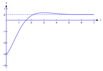
In Example 9.4.6 we found the inverse transform of this function to be

\[y={1\over2}-{7\over2}e^{-t}\cos t-{5\over2}e^{-t}\sin t \nonumber\]

(Figure 9.4.2 ), which is therefore the solution of Equation \ref{eq:8.3.15}.

Figure 9.4.2 : \(y=\frac{1}{2}-\frac{7}{2}e^{-t}\cos t-\frac{5}{2}e^{-t}\sin t\)

Example 9.4.8

Solve the initial value problem

\[\label{eq:8.3.16} y''-6y'+9y=t^2e^{3t}, \quad y(0)=2,\; y'(0)=6.\]

Solution

Taking Laplace transforms of both sides of the differential equation in Equation \ref{eq:8.3.16} yields

\[s^2Y(s)-sy(0)-y'(0)-6sY(s)+6y(0)+9Y(s)={2\over (s-3)^3}.\nonumber\]

This becomes

\[(s-3)^2Y(s)={2\over (s-3)^3}+2s-6.\nonumber\]

Solving for \(Y(s)\) yields

\[Y(s)={2\over (s-3)^5}+{2s\over (s-3)^2}-{6\over (s-3)^2}={1\over 12}{4!\over (s-3)^5}+{2(s-3)\over (s-3)^2}-{6\over (s-3)^2}={1\over 12}{4!\over (s-3)^5}+{2\over s-3}-{6\over (s-3)^2}.\nonumber\]

Taking the inverse Laplace transform gives us

\[y={1\over 12}t^4e^{3t}+2e^{3t}-3te^{3t}\nonumber\]

which is therefore the solution of Equation \ref{eq:8.3.16}.

Example 9.4.9

Solve the initial value problem

\[\label{eq:8.3.17} y''+4y'+6y=1+e^{-t}, \quad y(0)=0,\; y'(0)=0.\]

Solution

Taking Laplace transforms of both sides of the differential equation in Equation \ref{eq:8.3.17} yields

\[s^2Y(s)-sy(0)-y'(0)+4sY(s)-4y(0)+6Y(s)={1\over s}+{1\over s+1}.\nonumber\]

This becomes

\[[(s+2)^2+2]Y(s)={1\over s}+{1\over s+1}.\nonumber\]

Solving for \(Y(s)\) yields

\[Y(s)={1\over s[(s+2)^2+2]}+{1\over (s+1)[(s+2)^2+2]}={1/6\over s}+{1/3\over s+1}-{1\over 2}{s+2\over (s+2)^2+2}-{2\over 3}{1\over (s+2)^2+2}.\nonumber\]

Taking the inverse Laplace transform gives us

\[y={1\over 6}+{1\over 3}e^{-t}-{1\over 2}e^{-2t}\cos \sqrt {2}t-{\sqrt 2\over 3}e^{-2t}\sin \sqrt {2}t\nonumber\]

which is therefore the solution of Equation \ref{eq:8.3.17}.