8.E: Nonlinear Equations (Exercises)
- Last updated
- Save as PDF
- Page ID
- 32236
8.1: Linearization, critical points, and equilibria
Exercise \(\PageIndex{8.1.1}\)
Sketch the phase plane vector field for:
- \(x'=x^2, ~~y'=y^2\),
- \(x'=(x-y)^2, ~~y'=-x\),
- \(x'=e^y,~~ y'=e^x\).
Exercise \(\PageIndex{8.1.2}\)
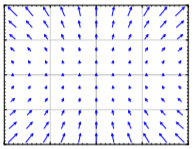
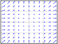
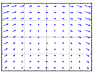
Match systems
- \(x'=x^2\), \(y'=y^2\),
- \(x'=xy\), \(y'=1+y^2\),
- \(x'=\sin(\pi y)\), \(y'=x\),
to the vector fields below. Justify.
Exercise \(\PageIndex{8.1.3}\)
Find the critical points and linearizations of the following systems.
- \(x'=x^2-y^2\), \(y'=x^2+y^2-1\),
- \(x'=-y\), \(y'=3x+yx^2\),
- \(x'=x^2+y\), \(y'=y^2+x\).
Exercise \(\PageIndex{8.1.4}\)
For the following systems, verify they have critical point at \((0,0)\), and find the linearization at \((0,0)\).
- \(x'=x+2y+x^2-y^2\), \(y'=2y-x^2\)
- \(x'=-y\), \(y'=x-y^3\)
- \(x'=ax+by+f(x,y)\), \(y'=cx+dy+g(x,y)\), where \(f(0,0) = 0\), \(g(0,0) = 0\), and all first partial derivatives of \(f\) and \(g\) are also zero at \((0,0)\), that is, \(\frac{\partial f}{\partial x}(0,0) = \frac{\partial f}{\partial y}(0,0) = \frac{\partial g}{\partial x}(0,0) = \frac{\partial g}{\partial y}(0,0) = 0\).
Exercise \(\PageIndex{8.1.5}\)
Take \(x'=(x-y)^2\), \(y'=(x+y)^2\).
- Find the set of critical points.
- Sketch a phase diagram and describe the behavior near the critical point(s).
- Find the linearization. Is it helpful in understanding the system?
Exercise \(\PageIndex{8.1.6}\)
Take \(x'=x^2\), \(y'=x^3\).
- Find the set of critical points.
- Sketch a phase diagram and describe the behavior near the critical point(s).
- Find the linearization. Is it helpful in understanding the system?
Exercise \(\PageIndex{8.1.7}\)
Find the critical points and linearizations of the following systems.
- \(x'=\sin(\pi y)+(x-1)^2\), \(y'=y^2-y\),
- \(x'=x+y+y^2\), \(y'=x\),
- \(x'=(x-1)^2+y\), \(y'=x^2+y\).
- Answer
-
- Critical points \((0, 0)\) and \((0, 1)\). At \((0, 0)\) using \(u=x\), \(v=y\) the linearization is \(u'=-2u-\left(\frac{1}{\pi}\right)v\), \(v'=-v\). At \((0, 1)\) using \(u=x\), \(v=y-1\) the linearization is \(u'=-2u+\left(\frac{1}{\pi}\right)v\) \(v'=v\).
- Critical point \((0, 0)\). Using \(u=x\), \(v=y\) the linearization is \(u'=u+v\), \(v'=u\).
- Critical point \(\left(\frac{1}{2},-\frac{1}{4}\right)\). Using \(u=x-\frac{1}{2}\), \(v=y+\frac{1}{4}\) the linearization is \(u'=-u+v\), \(v'=u+v\).
Exercise \(\PageIndex{8.1.8}\)
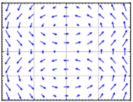
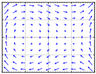
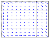
Match systems
- \(x'=y^2\), \(y'=-x^2\),
- \(x'=y\), \(y'=(x-1)(x+1)\),
- \(x'=y+x^2\), \(y'=-x\),
to the vector fields below. Justify.
- Answer
-
- is c),
- is a),
- is b)
Exercise \(\PageIndex{8.1.9}\)
The idea of critical points and linearization works in higher dimensions as well. You simply make the Jacobian matrix bigger by adding more functions and more variables. For the following system of 3 equations find the critical points and their linearizations:
\(x' = x + z^2,\quad y' = z^2-y, \quad z' = z+x^2.\)
- Answer
-
Critical points are \((0, 0, 0)\), and \((−1, 1, −1)\). The linearization at the origin using variables \(u=x\), \(v=y\), \(w=z\) is \(u'=u\), \(v'=-v\), \(z'=w\). The linearization at the point \((−1, 1, −1)\) using variables \(u=x+1\), \(v=y-1\), \(w=z+1\) is \(u'=u-2\), \(v'=-v-2w\), \(w'=w-2u\).
Exercise \(\PageIndex{8.1.10}\)
Any two-dimensional non-autonomous system \(x'=f(x,y,t)\), \(y'=g(x,y,t)\) can be written as a three-dimensional autonomous system (three equations). Write down this autonomous system using the variables \(u\), \(v\), \(w\).
- Answer
-
\(u'=f(u,v,w)\), \(v'=g(u,v,w)\), \(w'=1\).
8.2: Stability and classification of isolated critical points
Exercise \(\PageIndex{8.2.1}\)
For the systems below, find and classify the critical points, also indicate if the equilibria are stable, asymptotically stable, or unstable.
- \(x'=-x+3x^2, y'=-y\)
- \(x'=x^2+y^2-1\),\(y'=x\)
- \(x'=ye^x\),\(y'=y-x+y^2\)
Exercise \(\PageIndex{8.2.2}\)
Find the implicit equations of the trajectories of the following conservative systems. Next find their critical points (if any) and classify them.
- \(x''+ x+x^3 = 0\)
- \(\theta''+\sin \theta = 0\)
- \(z''+ (z-1)(z+1) = 0\)
- \(x''+ x^2+1 = 0\)
Exercise \(\PageIndex{8.2.3}\)
Find and classify the critical point(s) of \(x' = -x^2\),\(y' = -y^2\).
Exercise \(\PageIndex{8.2.4}\)
Suppose \(x'=-xy\),\(y'=x^2-1-y\).
- Show there are two spiral sinks at \((-1,0)\) and \((1,0)\).
- For any initial point of the form \((0,y_0)\),find what is the trajectory.
- Can a trajectory starting at \((x_0,y_0)\) where \(x_0 > 0\) spiral into the critical point at \((-1,0)\)? Why or why not?
Exercise \(\PageIndex{8.2.5}\)
In the example \(x'=y\),\(y'=y^3-x\) show that for any trajectory, the distance from the origin is an increasing function. Conclude that the origin behaves like is a spiral source. Hint: Consider \(f(t) = {\bigl(x(t)\bigr)}^2 + {\bigl(y(t)\bigr)}^2\) and show it has positive derivative.
Exercise \(\PageIndex{8.2.6}\)
Suppose \(f\) is always positive. Find the trajectories of \(x''+f(x') = 0\). Are there any critical points?
Exercise \(\PageIndex{8.2.7}\)
Suppose that \(x' = f(x,y)\),\(y' = g(x,y)\). Suppose that \(g(x,y) > 1\) for all \(x\) and \(y\). Are there any critical points? What can we say about the trajectories at \(t\) goes to infinity?
Exercise \(\PageIndex{8.2.8}\)
For the systems below, find and classify the critical points.
- \(x'=-x+x^2\),\(y'=y\)
- \(x'=y-y^2-x\),\(y'=-x\)
- \(x'=xy\),\(y'=x+y-1\)
- Answer
-
- \((0, 0)\): saddle (unstable), \((1, 0)\): source (unstable),
- \((0, 0)\): spiral sink (asymptotically stable), \((0, 1)\): saddle (unstable),
- \((1, 0)\): saddle (unstable), \((0, 1)\): source (unstable)
Exercise \(\PageIndex{8.2.9}\)
Find the implicit equations of the trajectories of the following conservative systems. Next find their critical points (if any) and classify them.
- \(x''+ x^2 = 4\)
- \(x''+ e^x = 0\)
- \(x''+ (x+1)e^x = 0\)
- Answer
-
- \(\frac{1}{2}y^{2}+\frac{1}{3}x^{3}-4x=C\), critical points: \((-2,0)\), an unstable saddle, and \((2,0)\), a stable center.
- \(\frac{1}{2}y^{2}+e^{x}=C\), no critical points.
- \(\frac{1}{2}y^{2}+xe^{x}=C\), critical point at \((-1,0)\) is a stable center.
Exercise \(\PageIndex{8.2.10}\)
The conservative system \(x''+x^3 = 0\) is not almost linear. Classify its critical point(s) nonetheless.
- Answer
-
Critical point at \((0, 0)\). Trajectories are \(y=\pm\sqrt{2C-\left(\frac{1}{2}\right)x^{4}}\), for \(C>0\), these give closed curves around the origin, so the critical point is a stable center.
Exercise \(\PageIndex{8.2.11}\)
Derive an analogous classification of critical points for equations in one dimension, such as \(x'= f(x)\) based on the derivative. A point \(x_0\) is critical when \(f(x_0) = 0\) and almost linear if in addition \(f'(x_0) \not= 0\). Figure out if the critical point is stable or unstable depending on the sign of \(f'(x_0)\). Explain. Hint: see Section 1.6.
- Answer
-
A critical point \(x_{0}\) is stable if \(f'(x_{0})<0\) and unstable when \(f'(x_{0})<0\).
8.3: Applications of nonlinear systems
Exercise \(\PageIndex{8.3.1}\)
Take the damped nonlinear pendulum equation \(\theta '' + \mu \theta' + (\frac{g}{L}) \sin \theta = 0\) for some \(\mu > 0\) (that is, there is some friction).
- Suppose \(\mu = 1\) and \(\frac{g}{L} = 1\) for simplicity, find and classify the critical points.
- Do the same for any \(\mu > 0\) and any \(g\) and \(L\), but such that the damping is small, in particular, \(\mu^2 < 4(\frac{g}{L})\).
- Explain what your findings mean, and if it agrees with what you expect in reality.
Exercise \(\PageIndex{8.3.2}\)
Suppose the hares do not grow exponentially, but logistically. In particular consider
\[x' = (0.4-0.01y)x - \gamma x^2, ~~~~~ y' = (0.003x-0.3)y .\]
For the following two values of \(\gamma\), find and classify all the critical points in the positive quadrant, that is, for \(x \geq 0\) and \(y \geq 0\). Then sketch the phase diagram. Discuss the implication for the long term behavior of the population.
- \(\gamma=0.001\),
- \(\gamma=0.01\).
Exercise \(\PageIndex{8.3.3}\)
- Suppose \(x\) and \(y\) are positive variables. Show \(\frac{y x}{e^{x+y}}\) attains a maximum at \((1,1)\).
- Suppose \(a,b,c,d\) are positive constants, and also suppose \(x\) and \(y\) are positive variables. Show \(\frac{y^a x^d}{e^{cx+by}}\) attains a maximum at \((\frac{d}{c},\frac{a}{b})\).
Exercise \(\PageIndex{8.3.4}\)
Suppose that for the pendulum equation we take a trajectory giving the spinning-around motion, for example \(\omega = \sqrt{\frac{2g}{L} \cos \theta + \frac{2g}{L} + \omega_0^2}\). This is the trajectory where the lowest angular velocity is \(\omega_0^2\). Find an integral expression for how long it takes the pendulum to go all the way around.
Exercise \(\PageIndex{8.3.5}\): (challenging)
Take the pendulum, suppose the initial position is \(\theta = 0\).
- Find the expression for \(\omega\) giving the trajectory with initial condition \((0,\omega_0)\). Hint: Figure out what \(C\) should be in terms of \(\omega_0\).
- Find the crucial angular velocity \(\omega_1\), such that for any higher initial angular velocity, the pendulum will keep going around its axis, and for any lower initial angular velocity, the pendulum will simply swing back and forth. Hint: When the pendulum doesn't go over the top the expression for \(\omega\) will be undefined for some \(\theta\)s.
- What do you think happens if the initial condition is \((0,\omega_1)\), that is, the initial angle is 0, and the initial angular velocity is exactly \(\omega_1\).
Exercise \(\PageIndex{8.3.6}\)
Take the damped nonlinear pendulum equation \(\theta '' + \mu \theta' + (\frac{g}{L}) \sin \theta = 0\) for some \(\mu > 0\) (that is, there is friction). Suppose the friction is large, in particular \(\mu^2 > 4 (\frac{g}{L})\).
- Find and classify the critical points.
- Explain what your findings mean, and if it agrees with what you expect in reality.
- Answer
-
- Critical points are \(\omega =0\), \(\theta =k\pi\) for any integer \(k\). When \(k\) is odd, we have a saddle point. When \(k\) is even we get a sink.
- The findings mean the pendulum will simply go to one of the sinks, for example \((0, 0)\) and it will not swing back and forth. The friction is too high for it to oscillate, just like an overdamped mass-spring system.
Exercise \(\PageIndex{8.3.7}\)
Suppose we have the system predator-prey system where the foxes are also killed at a constant rate \(h\) (\(h\) foxes killed per unit time): \(x' = (a-by)x,\) \(y' = (cx-d)y - h\).
- Find the critical points and the Jacobin matrices of the system.
- Put in the constants \(a=0.4\), \(b=0.01\), \(c=0.003\), \(d=0.3\), \(h=10\). Analyze the critical points. What do you think it says about the forest?
- Answer
-
- Solving for the critical points we get \((0,-\frac{h}{d})\) and \(\left(\frac{bh+ad}{ac},\frac{a}{b}\right)\). The Jacobian matrix at \((0,-\frac{h}{d})\) is \(\left[\begin{array}{cc}{a+\frac{bh}{d}}&{0}\\{-\frac{cd}{d}}&{-d}\end{array}\right]\) whose eigenvalues are \(a+\frac{bh}{d}\) and \(-d\). The eigenvalues are real of opposite signs and we get a saddle. (In the application, however, we are only looking at the positive quadrant so this critical point is irrelevant.) At \(\left(\frac{bh+ad}{ac},\frac{a}{b}\right)\) we get Jacobian matrix \(\left[\begin{array}{cc}{0}&{-\frac{b(bh+ad)}{ac}}\\{\frac{ac}{b}}&{\frac{bh+ad}{a}-d}\end{array}\right]\).
- For the specific numbers given, the second critical point is \(\left(\frac{550}{3},40\right)\) the matrix is \(\left[\begin{array}{cc}{0}&{-\frac{11}{6}}\\{\frac{3}{25}}&{\frac{1}{4}}\end{array}\right]\), which has eigenvalues \(\frac{5\pm\ i\sqrt{327}}{40}\). Therefore there is a spiral source; the solution spirals outwards. The solution eventually hits one of the axes, \(x=0\) or \(y=0\), so something will die out in the forest.
Exercise \(\PageIndex{8.3.8}\): (challenging)
Suppose the foxes never die. That is, we have the system \(x' = (a-by)x,\) \(y' = cxy\). Find the critical points and notice they are not isolated. What will happen to the population in the forest if it starts at some positive numbers. Hint: Think of the constant of motion.
- Answer
-
The critical points are on the line \(x=0\). In the positive quadrant the \(y'\) is always positive and so the fox population always grows. The constant of motion is \(C=y^{a}e^{-cx-by}\), for any \(C\) this curve must hit the \(y\)-axis (why?), so the trajectory will simply approach a point on the \(y\) axis somewhere and the number of hares will go to zero.
8.4: Limit cycles
Exercise \(\PageIndex{8.4.1}\)
Show that the following systems have no closed trajectories.
- \(x'=x^3+y,y'=y^3+x^2\),
- \(x'=e^{x-y},y'=e^{x+y}\),
- \(x'=x+3y^2-y^3,y'=y^3+x^2\).
Exercise \(\PageIndex{8.4.2}\)
Formulate a condition for a 2-by-2 linear system \({\vec{x}\,}' = A \vec{x}\) to not be a center using the Bendixson-Dulac theorem. That is, the theorem says something about certain elements of \(A\).
Exercise \(\PageIndex{8.4.3}\)
Explain why the Bendixson-Dulac Theorem does not apply for any conservative system \(x''+h(x) = 0\).
Exercise \(\PageIndex{8.4.4}\)
A system such as \(x'=x, y'=y\) has solutions that exist for all time \(t\), yet there are no closed trajectories or other limit cycles. Explain why the Poincare-Bendixson Theorem does not apply.
Exercise \(\PageIndex{8.4.5}\)
Differential equations can also be given in different coordinate systems. Suppose we have the system \(r' = 1-r^2\), \(\theta' = 1\) given in polar coordinates. Find all the closed trajectories and check if they are limit cycles and if so, if they are asymptotically stable or not.
Exercise \(\PageIndex{8.4.6}\)
Show that the following systems have no closed trajectories.
- \(x'=x+y^2\), \(y'=y+x^2\),
- \(x'=-x\sin^2(y)\), \(y'=e^x\),
- \(x'=xy\), \(y'=x+x^2\).
- Answer
-
Use Bendixson–Dulac Theorem.
- \(f_{x}+g_{y}=1+1>0\), so no closed trajectories.
- \(f_{x}+g_{y}=-\sin^{2}(y)+0<0\) for all \(x,y\) except the lines given by \(y=k\pi\) (where we get zero), so no closed trajectories.
- \(f_{x}+g_{y}=y+0>0\) for all \(x,y\) except the line given by \(y=0\) (where we get zero), so no closed trajectories.
Exercise \(\PageIndex{8.4.7}\)
Suppose an autonomous system in the plane has a solution \(x=\cos(t)+e^{-t}\), \(y=\sin(t)+e^{-t}\). What can you say about the system (in particular about limit cycles and periodic solutions)?
- Answer
-
Using Poincaré–Bendixson Theorem, the system has a limit cycle, which is the unit circle centered at the origin, as \(x=\cos (t)+e^{-t}\), \(y=\sin (t)+e^{-t}\) gets closer and closer to the unit circle. Thus \(x=\cos (t)\), \(y=\sin (t)\) is the periodic solution.
Exercise \(\PageIndex{8.4.8}\)
Show that the limit cycle of the Van der Pol oscillator (for \(\mu > 0\)) must not lie completely in the set where \(- \sqrt{\frac{1+\mu}{\mu}} < x < \sqrt{\frac{1+\mu}{\mu}}\). Compare with Figure 8.4.1.
- Answer
-
\(f(x,y)=y\), \(g(x,y)=\mu (1-x^{2})y-x\). So \(f_{x}+g_{y}=\mu (1-x^{2})\). The Bendixson–Dulac Theorem says there is no closed trajectory lying entirely in the set \(x^{2}<1\).
Exercise \(\PageIndex{8.4.9}\)
Suppose we have the system \(r' = \sin(r)\), \(\theta' = 1\) given in polar coordinates. Find all the closed trajectories.
- Answer
-
The closed trajectories are those where \(\sin (r)=0\), therefore, all the circles centered at the origin with radius that is a multiple of \(\pi\) are closed trajectories.
8.5: Chaos
Exercise \(\PageIndex{8.5.1}\)
For the non-chaotic equation \(x''+2p x' + \omega_0^2 x = \frac{F_0}{m} \cos (\omega t)\), suppose we strobe with frequency \(\omega\) as we mentioned above. Use the known steady periodic solution to find precisely the point which is the attractor for the Poincar\(\grave{e}\) section.
Exercise \(\PageIndex{8.5.2}\): (project)
A simple fractal attractor can be drawn via the following chaos game. Draw three points of a triangle (just the vertices) and number them, say \(p_1\), \(p_2\) and \(p_3\). Start with some random point \(p\) (does not have to be one of the three points above) and draw it. Roll a die, and use it to pick of the \(p_1\), \(p_2\), or \(p_3\) randomly (for example 1 and 4 mean \(p_1\), 2 and 5 mean \(p_2\), and 3 and 6 mean \(p_3\)). Suppose we picked \(p_2\), then let \(p_{\text{new}}\) be the point exactly halfway between \(p\) and \(p_2\). Draw this point and let \(p\) now refer to this new point \(p_{\text{new}}\). Rinse, repeat. Try to be precise and draw as many iterations as possible. Your points should be attracted to the so-called Sierpinski triangle. A computer was used to run the game for 10,000 iterations to obtain the picture in Figure \(\PageIndex{1}\).
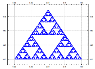
Figure \(\PageIndex{1}\): \(10,000\) iterations of the chaos game producing the Sierpinski triangle.
Exercise \(\PageIndex{8.5.3}\): (project)
Construct the double pendulum described in the text with a string and two nuts (or heavy beads). Play around with the position of the middle nut, and perhaps use different weight nuts. Describe what you find.
Exercise \(\PageIndex{8.5.4}\): (computer project)
Use a computer software (such as Matlab, Octave, or perhaps even a spreadsheet), plot the solution of the given forced Duffing equation with Euler's method. Plotting the solution for \(t\) from \(0\) to \(100\) with several different (small) step sizes. Discuss.
Exercise \(\PageIndex{8.5.5}\)
Find critical points of the Lorenz system and the associated linearizations.
- Answer
-
Critical points: \((0,0,0)\), \((3\sqrt{8},3\sqrt{8},27)\), \((-3\sqrt{8}, -3\sqrt{8}, 27)\). Linearization at \((0,0,0)\) using \(u=x\), \(v=y\), \(w=z\) is \(u'=-10u +10v\), \(v'=28u-v\), \(w'=-\left(\frac{8}{3}\right)w\). Linearization at \((3\sqrt{8}, 3\sqrt{8}, 27)\) using \(u=x-3\sqrt{8}\), \(v=y-3\sqrt{8}\), \(w=z-27\) is \(u'=-10u+10v\), \(v'=u-v-3\sqrt{8}w\), \(w'=3\sqrt{8}u+3\sqrt{8}v-\left(\frac{8}{3}\right) w\). Linearization at \((-3\sqrt{8}, -3\sqrt{8}, 27)\) using \(u=x+3\sqrt{8}\), \(v=y+3\sqrt{8}\), \(w=z-27\) is \(u'=-10u+10v\), \(v'=u-v+3\sqrt{8}w\), \(w'=-3\sqrt{8}u-3\sqrt{8}v-\left(\frac{8}{3}\right) w\).


