

5.6: Moments and Centers of Mass
- Page ID
- 212049

\( \newcommand{\vecs}[1]{\overset { \scriptstyle \rightharpoonup} {\mathbf{#1}} } \)
\( \newcommand{\vecd}[1]{\overset{-\!-\!\rightharpoonup}{\vphantom{a}\smash {#1}}} \)
\( \newcommand{\dsum}{\displaystyle\sum\limits} \)
\( \newcommand{\dint}{\displaystyle\int\limits} \)
\( \newcommand{\dlim}{\displaystyle\lim\limits} \)
\( \newcommand{\id}{\mathrm{id}}\) \( \newcommand{\Span}{\mathrm{span}}\)
( \newcommand{\kernel}{\mathrm{null}\,}\) \( \newcommand{\range}{\mathrm{range}\,}\)
\( \newcommand{\RealPart}{\mathrm{Re}}\) \( \newcommand{\ImaginaryPart}{\mathrm{Im}}\)
\( \newcommand{\Argument}{\mathrm{Arg}}\) \( \newcommand{\norm}[1]{\| #1 \|}\)
\( \newcommand{\inner}[2]{\langle #1, #2 \rangle}\)
\( \newcommand{\Span}{\mathrm{span}}\)
\( \newcommand{\id}{\mathrm{id}}\)
\( \newcommand{\Span}{\mathrm{span}}\)
\( \newcommand{\kernel}{\mathrm{null}\,}\)
\( \newcommand{\range}{\mathrm{range}\,}\)
\( \newcommand{\RealPart}{\mathrm{Re}}\)
\( \newcommand{\ImaginaryPart}{\mathrm{Im}}\)
\( \newcommand{\Argument}{\mathrm{Arg}}\)
\( \newcommand{\norm}[1]{\| #1 \|}\)
\( \newcommand{\inner}[2]{\langle #1, #2 \rangle}\)
\( \newcommand{\Span}{\mathrm{span}}\) \( \newcommand{\AA}{\unicode[.8,0]{x212B}}\)
\( \newcommand{\vectorA}[1]{\vec{#1}} % arrow\)
\( \newcommand{\vectorAt}[1]{\vec{\text{#1}}} % arrow\)
\( \newcommand{\vectorB}[1]{\overset { \scriptstyle \rightharpoonup} {\mathbf{#1}} } \)
\( \newcommand{\vectorC}[1]{\textbf{#1}} \)
\( \newcommand{\vectorD}[1]{\overrightarrow{#1}} \)
\( \newcommand{\vectorDt}[1]{\overrightarrow{\text{#1}}} \)
\( \newcommand{\vectE}[1]{\overset{-\!-\!\rightharpoonup}{\vphantom{a}\smash{\mathbf {#1}}}} \)
\( \newcommand{\vecs}[1]{\overset { \scriptstyle \rightharpoonup} {\mathbf{#1}} } \)
\(\newcommand{\longvect}{\overrightarrow}\)
\( \newcommand{\vecd}[1]{\overset{-\!-\!\rightharpoonup}{\vphantom{a}\smash {#1}}} \)
\(\newcommand{\ket}[1]{\left| #1 \right>}\)
\(\newcommand{\bra}[1]{\left< #1 \right|}\)
\(\newcommand{\braket}[2]{\left< #1 \vphantom{#2} \right| \left. #2 \vphantom{#1} \right>}\)
\(\newcommand{\braopket}[3]{\left< #1 \vphantom{#2}\vphantom{#3} \right| #2 \vphantom{#1}\vphantom{#3} \left| #3 \vphantom{#1}\vphantom{#2} \right>}\)
\(\newcommand{\qmvec}[1]{\mathbf{\vec{#1}}}\)
\(\newcommand{\op}[1]{\hat{\mathbf{#1}}}\)
\(\newcommand{\expect}[1]{\langle #1 \rangle}\)
\(\newcommand{\dfn}[1]{\emph{\textbf{#1}}}\)
This section develops a method for finding the center of mass of a thin, flat shape — the point at which the shape will balance without tilting:

Centers of mass are important because in many applied situations an object behaves as though its entire mass is located at its center of mass. For example, the work required to pump the water in a tank to a higher point is the same as the work required to move a small object with the same mass located at the tank’s center of mass to the higher point, a much easier problem (if we know the mass and the center of mass of the water):

Volumes and surface areas of solids of revolution can also become easy to calculate if we know the center of mass of the region being revolved.
Point-Masses in One Dimension
Before investigating the centers of mass of complicated regions, we consider point-masses (and systems of point-masses), first in one dimension and then in two dimensions.
Two people with different masses can position themselves on a seesaw so that the seesaw balances:

The person on the right causes the seesaw to “want to turn” clockwise about the fulcrum, and the person on the left causes it to “want to turn” counterclockwise. If these two “tendencies” are equal, the seesaw will balance on the fulcrum. A measure of this tendency to turn about the fulcrum is called the moment about the fulcrum of the system, and its magnitude is the product of the mass and the distance from the mass to the fulcrum. (In this seesaw example, we need to imagine that the seesaw is constructed using a very lightweight — yet sturdy — substance, so that its mass is negligible compared with the masses of the two people.)
In general, the moment about the origin, \(M_0\), produced by a mass \(m_1\) at a location \(x_1\) is \(m_1\cdot x_1\), the product of the mass and the “signed distance” of the point-mass from the origin:

For a system of \(n\) masses \(m_1\), \(m_2\),…, \(m_n\) at locations \(x_1\), \(x_2\), … , \(x_n\), respectively, the total mass of the system is:\[m = m_1 + m_2 + \cdots + m_n = \sum_{k=1}^n \, m_k\nonumber\]and the moment about the origin of the system is:\[M_0 = m_1\cdot x_1 + m_2\cdot x_2 + \cdots + m_n\cdot x_n = \sum_{k=1}^n \, m_k \cdot x_k\nonumber\]If the moment about the origin is positive, then the system “tends to rotate” clockwise about the origin. If the moment about the origin is negative, then the system “tends to rotate” counterclockwise about the origin. If the moment about the origin is zero, then the system does not tend to rotate in either direction about the origin: it balances on a fulcrum located at the origin.
The moment about a point \(\boldsymbol{x = p}\), \(M_p\), produced by a mass \(m_1\) at location \(x=x_1\) is the product of the mass and the signed distance of \(x_1\) from the point \(p\): \(m_1\cdot \left(x_1-p\right)\). The moment about a point \(x = p\) produced by masses \(m_1\), \(m_2\), … , \(m_n\) at locations \(x_1\), \(x_2\), … , \(x_n\), respectively, is:\[M_p = m_1\left(x_1-p\right) + m_2\left(x_2-p\right) + \cdots + m_n\left(x_n-p\right) = \sum_{k=1}^n \, m_k \left(x_k-p\right)\nonumber\]The point at which a system of point-masses balances is called the center of mass of the system, written \(\overline{x}\) (pronounced “\(x\)-bar”). Because the system balances at \(x = \overline{x}\), the moment about \(\overline{x}\), \(M_{\overline{x}}\), must be \(0\). (You have seen this “bar” notation before, in conjunction with the average value of a function. Here we can think of \(\overline{x}\) as a “weighted average.”)
Using this fact (and summation properties), we obtain a formula for \(\overline{x}\):
\begin{align*}0 &= M_{\overline{x}} = \sum_{k=1}^n \, m_k \cdot \left(x_k-\overline{x}\right) = \left[\sum_{k=1}^n \, m_k \cdot x_k\right] - \left[\sum_{k=1}^n \, m_k \cdot \overline{x}\right] \\
&= \left[\sum_{k=1}^n \, m_k \cdot x_k\right] - \overline{x}\cdot \left[\sum_{k=1}^n \, m_k\right] = M_0 - \overline{x}\cdot m\end{align*}
(we can factor \(\overline{x}\) out of the second sum because it is constant) so \(\overline{x}\cdot m = M_0\) and solving for \(\overline{x}\) yields the following formula.
The center of mass of a system of point-masses \(m_1\), \(m_2\), … , \(m_n\) at locations \(x_1\), \(x_2\),…, \(x_n\) is:\[\overline{x} = \frac{M_0}{m} = \frac{\sum_{k=1}^n \, m_k \cdot x_k}{\sum_{k=1}^n \, m_k}\nonumber\]
A single point-mass with mass \(m\) (the total mass of the system) located at \(\overline{x}\) (the center of mass of the system) produces the same moment about any point on the line as the whole system:
\begin{align*}M_p &= \sum_{k=1}^n\, m_k\left(x_k-p\right) = \left[\sum_{k=1}^n \, m_k x_k\right] - p\left[\sum_{k=1}^n\, m_k\right] = M_0 - pm\\
&= m\left(\frac{M_0}{m}-p\right) = m\left(\overline{x}-p\right)\end{align*}
For many purposes, we can think of the mass of the entire system as being “concentrated at \(\overline{x}\).”
Find the center of mass of the system consisting of the first three point-masses listed in the table below:
| \(k\) | \(m_k\) | \(x_k\) |
|---|---|---|
| 1 | 2 | -3 |
| 2 | 3 | 4 |
| 3 | 1 | 6 |
| 4 | 5 | -2 |
| 5 | 3 | 4 |
Solution
\(m = 2 + 3 + 1 = 6\) and \(M_0 = (2)(-3) + (3)(4) + (1)(6) = 12\) so:\[\overline{x} = \frac{M_0}{m} = \frac{12}{6} = 2\nonumber\]The system of three point-masses will balance on a fulcrum at \(x=2\).
Find the center of mass of the system consisting of the last three point-masses listed in the table from Example \(\PageIndex{1}\).
- Answer
-
\(m = 1 + 5 + 3 = 9\); \(M_0 = (1)(6) + (5)(-2) + (3)(4) = 8\); \mbox{\)\displaystyle \overline{x} = \frac{M_0}{m} = \frac89\);} the three point-masses will balance on a fulcrum located at \(\overline{x} = \frac89\).
Point-Masses in Two Dimensions
The concepts of moments and centers of mass extend nicely from one dimension to a system of masses located at points in a plane. For a “knife edge” fulcrum located along the \(y\)-axis:

the moment of a point-mass with mass \(m_1\) located at the point \(\left(x_1, y_1\right)\) is the product of the mass and the signed distance of the point-mass from the \(y\)-axis: \(m_1\cdot x_1\). This “tendency to rotate about the \(y\)-axis” is called the moment about the \(\boldsymbol{y}\)-axis, written \(M_y\). Here, \(M_y = m_1 \cdot x_1\). Similarly, a point-mass with mass \(m_1\) located at the point \(\left(x_1, y_1\right)\) has a moment about the \(\boldsymbol{x}\)-axis: \(M_x = m_1\cdot y_1\)

As in the seesaw example, we need to imagine that the point-masses are sitting on a thin — yet strong — plate of negligible mass compared with the point-masses.
For a system of masses \(m_k\) located at the points \(\left(x_k, y_k\right)\), the total mass of the system is (as before):\[m = m_1 + m_2 + \cdots + m_n = \sum_{k=1}^n \, m_k\nonumber\]while the moment about the \(y\)-axis is:\[M_y = m_1\cdot x_1 + m_2\cdot x_2 + \cdots + m_n\cdot x_n = \sum_{k=1}^n \, m_k \cdot x_k\nonumber\]and the moment about the \(x\)-axis is:\[M_x = m_1\cdot y_1 + m_2\cdot y_2 + \cdots + y_n\cdot x_n = \sum_{k=1}^n \, m_k \cdot y_k\nonumber\]At first, it may seem confusing that the formula for \(M_y\) would involve \(x\) and the formula for \(M_x\) would involve \(y\), but keep in mind that an equation for the \(y\)-axis is \(x=0\), so we could write the moment about the \(y\)-axis as \(M_{x=0}\) and the moment about the \(x\)-axis as \(M_{y=0}\).
The center of mass of this two-dimensional system is a point \(\left(\overline{x}, \overline{y}\right)\) such that any line that passes through this point is a “balancing fulcrum” for the system. So we need the moment about any such line — including \(x = \overline{x}\) and \(y = \overline{y}\) — to be zero:\[0 = M_{x=\overline{x}} = \sum_{k=1}^n \, m_k\left(x_k-\overline{x}\right) = \left[\sum_{k=1}^n \, m_k\cdot x_k\right] - \overline{x}\left[\sum_{k=1}^n \, m_k\right] = M_y - \overline{x}m\nonumber\]so \(\displaystyle \overline{x} = \frac{M_y}{m}\), and similar arithmetic shows that \(\displaystyle \overline{y} = \frac{M_x}{m}\).
If we can find such a point, then the system will balance on a single “point-fulcrum” located at the center of mass.
The center of mass of a system of point-masses \(m_1\), \(m_2\), … , \(m_n\) at locations \(\left(x_1, y_1\right)\), \(\left(x_2, y_2\right)\), … , \(\left(x_n, y_n\right)\) is the point \(\left(\overline{x}, \overline{y}\right)\) where:\[\overline{x} = \frac{M_y}{m} = \frac{\sum_{k=1}^n \, m_k \cdot x_k}{\sum_{k=1}^n \, m_k} \qquad \mbox{and} \qquad \overline{y} = \frac{M_x}{m} = \frac{\sum_{k=1}^n \, m_k \cdot y_k}{\sum_{k=1}^n \, m_k}\nonumber\]
A single point-mass with mass \(m\) (the total mass of the system) located at \(\left(\overline{x}, \overline{y}\right)\) (the center of mass of the system) produces the same moment about any line as the whole system does about that line. (The arithmetic needed to prove this statement is similar to arithmetic we did to prove the corresponding assertion for a one-dimensional system.) For many purposes, we can think of the mass of the entire system being “concentrated at \(\left(\overline{x}, \overline{y}\right)\).”
Find the center of mass of the system consisting of the first three point-masses listed in the table below:
| \(k\) | \(m_k\) | \(x_k\) | \(y_k\) |
|---|---|---|---|
| 1 | 2 | -3 | 4 |
| 2 | 3 | 4 | -7 |
| 3 | 1 | 6 | -2 |
| 4 | 5 | -2 | 1 |
| 5 | 3 | 4 | -6 |
Solution
\(m = 2 + 3 + 1 = 6\) and \(M_y = (2)(-3) + (3)(4) + (1)(6) = 12\) while \(M_x = (2)(4) + (3)(-7) + (1)(-2) = -15\) so:\[\overline{x} = \frac{M_y}{m} = \frac{12}{6} = 2 \qquad \mbox{and} \qquad \overline{y} = \frac{M_x}{m} = \frac{-15}{6} = -2.5\nonumber\]The system of three point-masses will balance on any fulcrum passing through the point \(\left(2, -2.5\right)\).
Find the center of mass of the system consisting of all five point-masses listed in the table from Example \(\PageIndex{2}\).
- Answer
-
\(m = 2 + 3 + 1 + 5 + 3 = 14\)
\(M_y = (2)(-3) + (3)(4) + (1)(6) + (5)(-2) + (3)(4) = 14\)
\(M_x = (2)(4) + (3)(-7) + (1)(-2) + (5)(1) + (3)(-6) = -28\)
\(\displaystyle \overline{x} = \frac{M_y}{m} = \frac{14}{14} = 1\) and \(\displaystyle \overline{y} = \frac{M_x}{m} = \frac{-28}{14} = -2\)
The five point-masses balance at the point \((1, -2)\).
Centroid of a Region
When we move from discrete point-masses to continuous regions in a plane, we move from finite sums and arithmetic to limits of Riemann sums, definite integrals and calculus. The following discussion extends ideas and calculations from point-masses to uniformly thin, flat plates (called lamina) that have a uniform density throughout (given as mass per area, such as “grams per cm\(^2\)”). The center of mass of one of these plates is the point \(\left(\overline{x}, \overline{y}\right)\) at which the plate balances without tilting.

It turns out that for plates with uniform density, the center of mass \(\left(\overline{x}, \overline{y}\right)\) depends only on the shape (and location) of the region of the plane covered by the plate and not on the (constant) density. In these uniform-density situations, we call the center of mass the centroid of the region. Throughout the following discussion, you should notice that each finite sum that appeared in the discussion of point-masses has an integral counterpart for these thin plates.

Rectangles
The components of a Riemann sum typically involve areas of rectangles, so it should come as no surprise that the basic shape used to extend point-mass concepts to regions is the rectangle. The total mass of a rectangular plate is the product of the area of the plate and its (constant) density: \(m = \mbox{mass} = \left(\mbox{area}\right)\cdot\left(\mbox{density}\right)\). We will assume that the center of mass of a thin, rectangular plate is located halfway up and halfway across the rectangle, at the point where the diagonals of the rectangle cross:

The moments of the rectangle about an axis can be found by treating the rectangle as a single point-mass with mass \(m\) located at the center of mass of the rectangle.
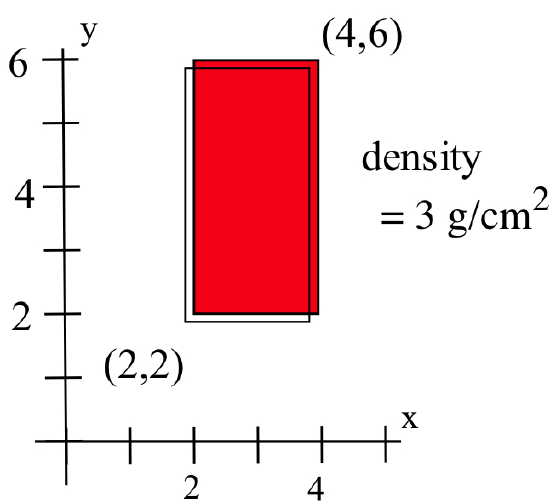
Find the moments about the \(x\)-axis, \(y\)-axis and the line \(x = 5\) of the thin, rectangular plate shown below:
Solution
The density of the plate is 3 g/cm\(^2\) and the area of the plate is \(\left(2\,\mbox{cm}\right)\left(4\,\mbox{cm}\right) = 8\,\mbox{cm}^2\) so the total mass is:\[m = \left (8\ \mbox{cm}^2\right)\left(3\ \frac{\mbox{g}}{\mbox{cm}^2}\right) = 24\ \mbox{g}\nonumber\]The center of mass of the rectangular plate is \(\left(\overline{x}, \overline{y}\right) = (3, 4)\). The moment about the \(x\)-axis is the product of the mass and the signed distance of the mass from the \(x\)-axis: \(M_x = \left(24\,\mbox{g}\right)\left(4\,\mbox{cm}\right) = 96\,\mbox{g-cm}\). Similarly, \(M_y = \left(24\,\mbox{g}\right)\left(3\,\mbox{cm}\right) = 72\,\mbox{g-cm}\). The moment about the line \(x = 5\) is \(M_{x=5} = \left(24\,\mbox{g}\right)\left(\left[5-3\right]\,\mbox{cm}\right) = 48\,\mbox{g-cm}\).
To find the moments and center of mass of a plate made up of several rectangular regions, we can simply treat each of the rectangular pieces as a point-mass concentrated at its center of mass, then treat the plate as a system of discrete point-masses.
Find the centroid of the region in the figure below:

Solution
We can divide the plate into two rectangular plates, one with mass \(24\ \mbox{g}\) and center of mass \((1,4)\), and the other with mass \(12\ \mbox{g}\) and center of mass \((3,3)\). The total mass of the pair of point-masses is \(m = 24+12 = 36\ \mbox{g}\), and the moments about the axes are \(M_x = \left(24\ \mbox{g}\right)\left(4\ \mbox{cm}\right) + \left(12\ \mbox{g}\right)\left(3\ \mbox{cm}\right) = 132 \ \mbox{g-cm}\) and \(M_y = \left(24\ \mbox{g}\right)\left(1\ \mbox{cm}\right) + \left(12\ \mbox{g}\right)\left(3\ \mbox{cm}\right) = 60 \ \mbox{g-cm}\). So:\[\overline{x} = \frac{M_y}{m} = \frac{60 \ \mbox{g-cm}}{36 \ \mbox{g}} = \frac53 \ \mbox{cm} \quad \mbox{and} \quad \overline{y} = \frac{M_x}{m} = \frac{132 \ \mbox{g-cm}}{36 \ \mbox{g}} = \frac{11}{3} \ \mbox{cm}\nonumber\]The centroid of the plate is located at \(\left(\frac53, \frac{11}{3}\right)\).
Find the centroid of the region in the figure below:

- Answer
-
There are several ways to break the region into “easy” pieces — one way is to consider the four 2 cm-by-2 cm squares. The center of mass of each square is located at the center of the square (at \((2,2)\), \((4,2)\), \((6,2)\) and \((4,4)\)), and each square has mass \(\left(4\ \mbox{cm}^2\right)\left(5\ \frac{\mbox{g}}{\mbox{cm}^2}\right) = 20\ \mbox{g}\) so: \(m = 4\left(20\, \mbox{g}\right) = 80\, \mbox{g}\), \)M_y = 2(20) + 4(20) + 6(20) + 4(20) = 320\, \mbox{g-cm}\) and \(M_x = 2(20) + 2(20) + 2(20) + 4(20) = 200\ \mbox{g-cm}\). Therefore \(\displaystyle \overline{x} = \frac{M_y}{m} = \frac{320\ \mbox{g-cm}}{80\ \mbox{g}} = 4 \ \mbox{cm}\) and \(\displaystyle \overline{y} = \frac{M_x}{m} = \frac{200\ \mbox{g-cm}}{80\ \mbox{g}} = 2.5 \ \mbox{cm}\) so the center of mass is located at \((4, 2.5)\).
To find the center of mass of a thin, non-rectangular plate, we will “slice” the plate into narrow, almost-rectangular plates and treat the collection of almost-rectangular plates as a system of point-masses located at the centers of mass of the almost-rectangles. The total mass and moments about the axes for the system of point-masses will be Riemann sums. By taking limits as the widths of the almost-rectangles approach \(0\), we will obtain exact values for the mass and moments as definite integrals.
\(\overline{x}\) for a Region
Suppose \(f(x) \geq g(x)\) on the interval \([a,b]\) and \(\cal{R}\) is a plate of uniform density (\(=\rho\)) sitting on the region between the graphs of \(f(x)\) and \(g(x)\) and the lines \(x=a\) and \(x=b\):

If we partition the interval \([a, b]\) into \(n\) subintervals of the form \(\left[x_{k-1}, x_k\right]\) and choose the points \(c_k\) to be the midpoints of these subintervals, then the slice between vertical cuts at \(x = x_{k-1}\) and \(x = x_k\) is approximately rectangular and has mass approximately equal to:
\begin{align*}\left(\mbox{area}\right)\left(\mbox{density}\right) &= \left(\mbox{height}\right)\left(\mbox{width}\right)\left(\mbox{density}\right)\\
&\approx \left[f\left(c_k\right) - g\left(c_k\right)\right]\cdot\left(x_{k-1} - x_k\right) \cdot \rho\\
&= \rho \left[f\left(c_k\right) - g\left(c_k\right)\right] \Delta x_k\end{align*}
So the mass of the whole plate is approximately\[m = \sum_{k=1}^n \, \rho \left[f\left(c_k\right) - g\left(c_k\right)\right] \Delta x_k \ \longrightarrow \ \int_a^b \rho \left[f(x)-g(x)\right] \, dx = \rho \cdot A\nonumber\]where \(A\) is the area of the region \(\cal{R}\).
(The Greek letter \(\rho\) (pronounced “row,” as in “row your boat”) is often used to represent the density of a region.)
The moment about the \(y\)-axis of each almost-rectangular slice is the product of the mass of the slice (\(m\)) and the distance from the centroid of the almost-rectangle to the \(y\)-axis. The \(x\)-coordinate of that centroid is located at \(x = c_k\), so the distance from the centroid to the \(y\)-axis is \(c_k-0=c_k\). The moment of the almost-rectangle about the \(y\)-axis is therefore:\[m_k\cdot c_k = \left(\rho \left[f\left(c_k\right) - g\left(c_k\right)\right] \Delta x_k \right)\cdot c_k\nonumber\]so the moment of the entire plate about the \(y\)-axis is (approximately):\[M_y = \sum_{k=1}^n \, \rho c_k \cdot \left[f\left(c_k\right) - g\left(c_k\right)\right] \Delta x_k \ \longrightarrow \ \int_a^b \rho x\cdot \left[f(x)-g(x)\right] \, dx\nonumber\]The \(x\)-coordinate of the centroid of the plate is therefore:\[\overline{x} = \frac{M_y}{m} = \frac{\rho \int_a^b x\cdot\left[f(x)-g(x)\right]\, dx}{\rho \int_a^b \left[f(x)-g(x)\right]\, dx} = \frac{\int_a^b x\cdot\left[f(x)-g(x)\right]\, dx}{\int_a^b \left[f(x)-g(x)\right]\, dx}\nonumber\]The density constant \(\rho\) is a factor of both \(M_y\) and \(m\), so it cancels and has no effect on the value of \(\overline{x}\). The value of \(\overline{x}\) depends only on the shape and location of the region \(\cal{R}\).
If the bottom boundary of \(\cal{R}\) is the \(x\)-axis, then \(g(x) = 0\) and the previous formulas simplify to:\[m = \rho \int_a^b f(x) \, dx{,} \ \ M_y = \rho \int_a^b x f(x) \, dx \ \ \mbox{and} \ \ \overline{x} = \frac{M_y}{m} = \frac{\int_a^b x f(x)\, dx}{\int_a^b f(x)\, dx}\]
Find the \(x\)-coordinate of the centroid of the region between \(f(x) = x^2\), the \(x\)-axis and \(x = 2\).
- Answer
-
For simplicity, let \(\rho =1\). Then the mass is \(\displaystyle m = \int_0^2 x^2\, dx = \frac83\) while \)\displaystyle M_y = \int_0^2 x\cdot x^2 \, dx = \int_0^2 x^3 \, dx = 4\) so \)\displaystyle \overline{x} = \frac{4}{\frac83} = \frac32 = 1.5\).
\(\overline{y}\) for a Region
To find \(\overline{y}\), the \(y\)-coordinate of the centroid of \(\cal{R}\), we need to find \(M_x\), the moment of \(\cal{R}\) about the \(x\)-axis. For vertical partitions of \(\cal{R}\):

the moment of each narrow strip about the \(x\)-axis, \(M_x\), is the product of the strip's mass and the signed distance between the centroid of the strip and the \(x\)-axis. We've already computed the mass:\[m_k = \rho \left[f\left(c_k\right) - g\left(c_k\right)\right] \Delta x_k\nonumber\]Because each strip is nearly rectangular, the centroid of the \(k\)-th strip is roughly halfway up the strip, at a point midway between \(f\left(c_k\right)\) and \(g\left(c_k\right)\), so we can average those function values to compute:\[\overline{y}_k \approx \frac{f\left(c_k\right) + g\left(c_k\right)}{2}\nonumber\]The moment about the \(x\)-axis for this strip is thus:\[\rho \left[f\left(c_k\right) - g\left(c_k\right)\right] \Delta x_k \cdot\left[\frac{f\left(c_k\right) + g\left(c_k\right)}{2}\right] = \frac{\rho}{2}\left[\left(f\left(c_k\right)\right)^2 - \left(g\left(c_k\right)\right)^2\right]\Delta x_k\nonumber\]Adding up the moments of all \(n\) strips yields:\[M_x = \sum_{k=1}^n \, \frac{\rho}{2}\left[\left(f\left(c_k\right)\right)^2 - \left(g\left(c_k\right)\right)^2\right]\Delta x_k \longrightarrow \int_a^b \frac{\rho}{2}\left[\left(f\left(x\right)\right)^2 - \left(g\left(x\right)\right)^2\right] \, dx\nonumber\]The \(y\)-coordinate of the centroid of the plate is therefore:\[\overline{y} = \frac{M_x}{m} = \frac{\rho \int_a^b \frac12 \left[\left(f\left(x\right)\right)^2 - \left(g\left(x\right)\right)^2\right]\, dx}{\rho \int_a^b \left[f(x)-g(x)\right]\, dx} = \frac{\int_a^b \frac12 \left[\left(f\left(x\right)\right)^2 - \left(g\left(x\right)\right)^2\right]\, dx}{\int_a^b \left[f(x)-g(x)\right]\, dx}\nonumber\]If the bottom boundary of \(\cal{R}\) is the \(x\)-axis, then \(g(x) = 0\) and the previous formulas simplify to:\[M_x = \frac{\rho}{2} \int_a^b x \left[f(x)\right]^2 \, dx \ \ \mbox{and} \ \ \overline{y} = \frac{M_x}{m} = \frac{\int_a^b \frac12 \left[f(x)\right]^2\, dx}{\int_a^b f(x)\, dx}\nonumber\]
Find the \(y\)-coordinate of the centroid of the region \(\cal{R}\) bounded below by the \(x\)-axis and above by the top half of a circle of radius \(r\) centered at the origin:

Solution
An equation for the circle is \(x^2 + y^2 = r^2\) so the top half is given by \(f(x) = y = \sqrt{r^2-x^2}\), and \(g(x) = 0\). The mass of the region is:\[m = \int_{-r}^{r} \rho \sqrt{r^2-x^2}\, dx = \rho \int_{-r}^{r} \sqrt{r^2-x^2}\, dx = \rho \cdot\left[\mbox{area of }\cal{R}\right] = \rho \cdot \frac{\pi r^2}{2}\nonumber\]The moment of \(\cal {R}\) about the \(y\)-axis is:\[M_y = \int_{-r}^{r} \rho x \cdot \sqrt{r^2-x^2}\, dx = \left[-\frac{\rho}{3}\left(r^2-x^2\right)^{\frac32}\right]_{x = -r}^{x= r} = 0\nonumber\]so \(\overline{x} = 0\). (Could you have guessed this result merely by looking at the region?)
The moment of \(\cal {R}\) about the \(x\)-axis is:
\begin{align*}M_x &= \int_{-r}^{r} \frac{\rho}{2} \cdot \left[\sqrt{r^2-x^2}\right]^2 \, dx = \frac{\rho}{2} \int_{-r}^{r} \left[r^2-x^2\right] \, dx\\
&= \frac{\rho}{2} \left[r^2 x -\frac13 x^3\right]_{-r}^{r} = \frac{\rho}{2} \cdot \frac43 r^3 = \frac{2\rho}{3}r^3\end{align*}
so \(\displaystyle \overline{y} = \frac{\frac{2\rho}{3}r^3}{\frac{\rho\pi}{2}r^2} = \frac{4}{3\pi}r \approx 0.4244r\). (Could you have guessed that centroid would be located a bit less than halfway above the bottom edge of the semicircle, merely by looking at the region?)
Show that the centroid of a triangular region with vertices \((0,0)\), \((0,h)\) and \((b,0)\) is located at \(\displaystyle \left(\overline{x}, \overline{y}\right) = \left(\frac{b}{3}, \frac{h}{3}\right)\).
- Answer
-
The triangular region appears below:

Here \(\displaystyle f(x) = h - \frac{h}{b}x\) for \(0 \leq x \leq b\) and \(g(x) = 0\). The “mass” is just the area of the triangle, so \(m = \frac12 \cdot b \cdot h\) while:\[M_y = \int_0^b x\left[h - \frac{h}{b}x\right]\, dx = \int_0^b \left[hx - \frac{h}{b}x^2\right]\, dx = \left[\frac{h}{2}x^2 - \frac{h}{3b}x^3\right]_0^b = \frac{b^2h}{6}\nonumber\]and:\[M_x = \int_0^b \frac12\left[h - \frac{h}{b}x\right]^2 \, dx = \left[\frac16\left(-\frac{b}{h}\right)\left(h - \frac{h}{b}x\right)^3\right]_0^b = 0 + \frac{b}{6h}\cdot h^3 = \frac{bh^2}{6}\nonumber\]So \(\displaystyle \left(\overline{x}, \overline{y}\right) = \left(\frac{\frac{b^2h}{6}}{\frac{bh}{2}},\frac{\frac{bh^2}{6}}{\frac{bh}{2}}\right) = \left(\frac{b}{3}, \frac{h}{3}\right)\).
The following table summarizes and compares formulas for computing moments and centers of mass for a system of point-masses in a plane (using sums) and for a region in a plane (using integrals). The integral formulas appear in a form for calculating moments of a region \(\cal{R}\) bounded by the graphs of two functions, \(f(x)\) and \(g(x)\), and two vertical lines, \(x = a\) and \(x = b\), where \(f(x) \geq g(x)\) for \(a \leq x \leq b\).
| point-masses in plane | region \(\boldsymbol {\cal R}\) between \(\boldsymbol{f}\) and \(\boldsymbol{g}\) | |
|---|---|---|
| total mass: | \(\displaystyle m = \sum_{k=1}^n \, m_k\) | \(\displaystyle m = \int_a^b \rho \left[f(x)-g(x)\right] \, dx = \rho\cdot\mbox{Area}\left({\cal R}\right)\) |
| moment about \(y\)-axis (\(x=0\)): | \(\displaystyle M_y = \sum_{k=1}^n \, m_k\cdot x_k\) | \(\displaystyle M_y = \int_a^b \rho x\cdot \left[f(x)-g(x)\right] \, dx\) |
| moment about \(x\)-axis (\(y=0\)): | \(\displaystyle M_x = \sum_{k=1}^n \, m_k\cdot y_k\) | \(\displaystyle M_x = \int_a^b \frac{\rho}{2} \left[\left(f(x)\right)^2-\left(g(x)\right)^2\right] \, dx\) |
| center of mass (\(\rho\) constant): | \(\displaystyle \overline{x} = \frac{M_y}{m}, \ \overline{y} = \frac{M_x}{m}\) | \(\displaystyle \overline{x} = \frac{M_y}{m}, \ \overline{y} = \frac{M_x}{m}\) |
While the integral formulas above are often useful, it is important that you understand the process used to obtain these formulas in order to compute moments and centroids of more general regions. (With the knowledge of Riemann sums you have developed, you should be able to set up integrals to compute masses and moments for regions bounded by curves of the form \(x = g(y)\), and deal with situations where the density of a thin plate is a function of \(x\) or \(y\).)
Find the centroid of the region \(\cal{R}\) bounded by the graphs of \(y = x^2\) and \(y = x^3\):

Solution
The curves intersect where \(x^2=x^3 \Rightarrow x^2-x^3=0 \Rightarrow x^2(1-x)=0 \Rightarrow x = 0\) or \(x = 1\). A graph (see margin) helps confirm that \(x^2 \geq x^3\) on \(\left[0, 1\right]\). If the density of \(\cal{R}\) is \(\rho\) then the mass of \(\cal{R}\) is:\[m = \int_0^1 \rho \left[x^2-x^3\right]\, dx = \rho\left[\frac13 x^3 - \frac14 x^4\right]_0^1 = \frac{\rho}{12}\nonumber\]The moment of \(\cal{R}\) about the \(y\)-axis is:\[M_y = \rho \int_0^1 x\left[x^2-x^3\right]\, dx = \rho \int_0^1 \left[x^3-x^4\right]\, dx = \rho\left[\frac14 x^4 - \frac15 x^5\right]_0^1 =\frac{\rho}{20}\nonumber\]And the moment of \(\cal{R}\) about the \(x\)-axis is:\[M_x = \frac{\rho}{2} \int_0^1 \left[\left(x^2\right)^2-\left(x^3\right)^2\right]\, dx = \frac{\rho}{2} \left[\frac15 x^5 - \frac17 x^7\right]_0^1 = \frac{\rho}{35}\nonumber\]so \(\displaystyle \overline{x} = \frac{M_y}{m} = \frac{\frac{\rho}{20}}{\frac{\rho}{12}} = \frac35\) and \(\displaystyle \overline{y} = \frac{M_x}{m} = \frac{\frac{\rho}{35}}{\frac{\rho}{12}} = \frac{12}{35}\). Plotting the point \(\left(\frac35, \frac{12}{35}\right) \approx \left(0.60, 0.34\right)\) along with \(\cal{R}\) confirms that it sits inside \(\cal{R}\) (just barely) and appears to be a reasonable candidate for the centroid.
Symmetry
Symmetry is a very powerful geometric concept that can simplify many mathematical and physical problems, including the task of finding centroids of regions. For some regions, we can use symmetry alone to determine the centroid. Geometrically, a region \(\cal{R}\) is symmetric about a line \(\boldsymbol{L}\) if, when \(\cal{R}\) is folded along \(L\), each point of \(\cal{R}\) on one side of the fold matches up with exactly one point of \(\cal{R}\) on the other side of the fold:

Sketch two lines of symmetry for each region shown in the figure below:

Solution
See solution to Practice \(\PageIndex{6}\).
A very useful fact about symmetric regions is that the centroid \(\left(\overline{x}, \overline{y}\right)\) of a symmetric region must lie on every line of symmetry of the region.
(In Example , the half-disk was symmetric with respect to the \(y\)-axis, so we could have avoided setting up and evaluating the \(M_y\) integral by noticing that \(\left(\overline{x}, \overline{y}\right)\) must be located on the \(y\)-axis (the line \(x=0\)) and concluding that \(\overline{x} = 0\).} If a region has two different lines of symmetry, then the centroid must lie on each of them, so the centroid must be located at the point where the lines of symmetry intersect.)
Locate the centroid of each region in Example \(\PageIndex{7}\).
- Answer
-
The centroid of each region is located at the point where the lines of symmetry intersect:

Work
In a uniform gravitational field, the center of gravity of an object is located at the same point as its center of mass, and the work done to lift an object is the product of the object’s weight and the distance that the center of gravity of the object is raised:\[\mbox{work} = \left(\mbox{object's weight}\right)\left(\mbox{distance object's center of gravity is raised}\right)\nonumber\]In the high jump, this explains the effectiveness of the “Fosbury Flop,” a technique where the jumper assumes an inverted U position while going over the bar:

The jumper’s body goes over the bar while the jumper’s center of gravity goes under it, allowing the jumper to clear a higher bar with no additional upward thrust.
If you know the center of gravity of an object being lifted, some work problems become much easier.
The trough shown below is filled with a liquid weighing 70 pounds per cubic foot:

How much work is done pumping the liquid over the wall next to the trough?
Solution
(We’ve already solved this problem, as Example 5 in Section 5.4, but here we try a new approach using centroids.)
This is a 3-D problem, but symmetry tells us the centroid of the liquid must be at a point 2.5 feet from either end of the trough, and 1 foot away from the wall. The vertical coordinate of the centroid will be the same as the centroid of the trough's triangular end region.
Using the result of Practice \(\PageIndex{5}\), we can conclude that the centroid of the triangle is at a height of \(\frac23 \cdot 4 = \frac83\). The weight of the liquid is:\[\left(\mbox{density}\right)\cdot\left(\mbox{volume}\right) = \left(70 \ \frac{\mbox{lb}}{\mbox{ft}^3}\right)\cdot\frac12\left(5\ \mbox{ft}\right)\cdot\left(2\ \mbox{ft}\right)\cdot\left(4\ \mbox{ft}\right) = 1400 \ \mbox{lbs}\nonumber\]and the distance the center of gravity must be moved is \(\displaystyle 6 - \frac{8}{3} = \frac{10}{3} \ \mbox{ft}\) so the total work required is:\[\left(1400 \ \mbox{lbs}\right)\cdot\left(\frac{10}{3} \ \mbox{ft}\right) = \frac{14000}{3} \ \mbox{ft-lbs} \approx 4666.7 \ \mbox{ft-lbs}\nonumber\]which agrees with the answer obtained in Section 5.4.
Theorems of Pappus
Two theorems due to Pappus of Alexandria can make some volume and surface area calculations relatively easy. (Pappus, the last of the great Greek geometers, flourished during the first half of the fourth century.)
If: a plane region \(\cal{R}\) with area \(A\) and centroid \(\displaystyle \left(\overline{x}, \overline{y}\right)\) is revolved around a line \(L\) in the plane that does not pass through \(\cal{R}\) (touching the boundary is OK)
then: the volume swept out by one revolution of \(\cal{R}\) is the product of \(A\) and the distance traveled by the centroid.
The distance from the centroid to the line will be the radius of the circle swept out by the centroid, so the distance traveled by the centroid is \(2\pi\) times this radius. When \(L\) is the \(x\)-axis, the volume of the solid is \(A\cdot 2\pi\overline{y}\); when \(L\) is the \(y\)-axis, the volume of the solid is \(A\cdot 2\pi\overline{x}\).

Find the volume swept out when the region \(\cal{R}\) bounded by the graphs of \(y = x^2\) and \(y = x^3\) is revolved around the line \(x=2\).
Solution
From Example 6, we know the area of \(\cal{R}\) is \(\frac{1}{12}\) and its centroid is \(\left(\frac35, \frac{12}{35}\right)\). The distance from this point to the line \(x=2\) is \(2-\frac35 = \frac75\), so the distance traveled by the centroid is \(\displaystyle 2\pi\cdot\frac75 = \frac{14\pi}{5}\). The volume of the solid of revolution is therefore \(\displaystyle \frac{1}{12}\cdot\frac{14\pi}{5} = \frac{7\pi}{30}\).
If: a plane region \(\cal{R}\) with perimeter \(P\) and centroid \(\displaystyle \left(\overline{x}, \overline{y}\right)\) is revolved around a line \(L\) in the plane that does not pass through \(\cal{R}\) (touching the boundary is OK)
then: the surface area swept out by one revolution of \(\cal{R}\) is the product of \(P\) and the distance traveled by the centroid.
When \(L\) is the \(x\)-axis, the surface area of the solid is \(P\cdot 2\pi\overline{y}\); when \(L\) is the \(y\)-axis, the surface area is \(P\cdot 2\pi\overline{x}\).

Find the surface area of the solid swept out when the square region \(\cal{R}\) with vertices at \((1,0)\), \((0,1)\), \((-1,0)\) and \((0,-1)\) is revolved around the line \(y=3\).
Solution
By symmetry, the centroid of the square is \((0,0)\) and its distance from \(y=3\) is \(3\). The perimeter of the square is \(4\sqrt{2}\), so the surface area of the solid of revolution is \(4\sqrt{2}\cdot 2\pi\cdot 3 = 24\pi\sqrt{3}\).
Problems
-
- Find the total mass and the center of mass for a system consisting of the three point-masses in the table below:
\(m_k\) 2 5 5 \(x_k\) 4 2 6 - Where should you locate a new object with mass \(8\) so the new system has its center of mass at \(x = 5\)?
- What mass should you put at \(x = 10\) so the original system plus the new mass has its center of mass at \(x = 6\)?
- Find the total mass and the center of mass for a system consisting of the three point-masses in the table below:
-
- Find the total mass and the center of mass for a system consisting of the four point-masses in the table below:
\(m_k\) 5 3 2 6 \(x_k\) 1 7 5 5 - Where should you locate a new object with mass \(10\) so the new system has its center of mass at \(x = 6\)?
- What mass should you put at \(x = 14\) so the original system plus the new mass has its center of mass at \(x = 6\)?
- Find the total mass and the center of mass for a system consisting of the four point-masses in the table below:
-
- Find the total mass and the center of mass for a system consisting of the three point-masses in the table below.
\(m_k\) 2 5 5 \(x_k\) 4 2 6 \(y_k\) 3 4 2 - Where should you locate a new object with mass \(10\) so the new system has its center of mass at \((5,2)\)?
- Find the total mass and the center of mass for a system consisting of the three point-masses in the table below.
-
- Find the total mass and the center of mass for a system consisting of the four point-masses in the table below.
\(m_k\) 5 3 2 6 \(x_k\) 1 7 5 5 \(y_k\) 4 7 0 8 - Where should you locate a new object with mass \(12\) so the new system has its center of mass at \((3,5)\)?
- Find the total mass and the center of mass for a system consisting of the four point-masses in the table below.
In Problems 5–10, divide the plate shown into rectangles and semicircles, calculate the mass, moments and centers of mass of each piece, then find the center of mass of the plate. Assume the density of the plate is \(\rho = 1\). Plot the location of the center of mass for each shape. (Refer to Example \(\PageIndex{5}\) for centroids of semicircular regions.)
- Use the figure below left.

- Use the figure above right.
- Use the figure below left.

- Use the figure above right.
- Use the figure below left.

- Use the figure above right.
In Problems 11–26, sketch the region bounded by the the given curves and find the centroid of each region (use technology to evaluate integrals, if necessary). Plot the location of the centroid on your sketch of the region.
- \(y = x\), the \(x\)-axis, \(x = 3\)
- \(y = x^2\), the \(x\)-axis, \(x=-2\), \(x = 2\)
- \(y = x^2\), \(y = 4\)
- \(y = \sin(x)\), the \(x\)-axis, the \(y\)-axis, \(x=\pi\)
- \(y = 4 - x^2\) and the \(x\)-axis for \(-2 \leq x \leq 2\)
- \(y = x^2\), \(y = x\)
- \(y = 9 - x\), \(y = 3\), \(x=0\), \(x=3\)
- \(y = \sqrt{1 - x^2}\), the \(x\)-axis, \(x=0\), \(x=1\)
- \(y = \sqrt{x}\), the \(x\)-axis, \(x=9\)
- \(y = \ln(x)\), the \(x\)-axis, \(x=e\)
- \(y = e^x\), \(y = e\) and the \(y\)-axis
- \(y = x^2\) and \(y = 2x\)
- An empty box in the shape of a cube measuring 1 foot on each side weighs 10 pounds. By symmetry, we know its center of mass is 6 inches above its bottom. When the box is full of a liquid with density 60 lb/ft\(^3\), the center of mass of the box-liquid system is again (due to symmetry) 6 inches above the bottom of the box.
- Find the height of the center of mass of the box-liquid system as a function of \(h\), the height of water in the box.
- To what height should you fill the box so that the box-liquid system has the lowest center of gravity (and the greatest stability)?
- The empty glass shown below left has a mass of 100 g when empty. Find the height of the center of mass of the glass-water system as a function of the height of water in the glass.

- The empty soda can shown above right has a mass of 15 g when empty and 400 g when full of soda. Find the height of the center of mass of the can-soda system as a function of the height of the soda in the can.
- Give a practical set of directions someone could actually use to find the height of the center of gravity of their body with their arms at their sides. How will the height of the center of gravity change if they lift their arms?
- Try the following experiment. Stand straight with your back and heels against a wall. Slowly raise one leg, keeping it straight, in front of you. What happened? Why?
- Why can’t two dancers stand in the position shown below?

- If a shape has exactly two lines of symmetry, the lines can meet at right angles. Must they meet at right angles?
- Sketch regions with exactly two lines of symmetry, exactly three lines of symmetry, and exactly four lines of symmetry.
- A rectangular box is filled to a depth of 4 feet with 300 pounds of water. How much work is done pumping the water to a point 10 feet above the bottom of the box?
- A cylinder is filled to a depth of 2 feet with 40 pounds of water. How much work is done pumping the water to a point 7 feet above the bottom of the cylinder?
- A sphere of radius 2 m is filled with water. How much work is done pumping the water to a point 3 m above the top of the sphere?
- A sphere of radius 2 feet is filled with water. How much work is done pumping the water to a point 5 feet above the top of the sphere?
- The center of a square region with sides of length 2 cm is located at the point \((3,4)\). Find the volume swept out when the square region is rotated:
- about the \(x\)-axis.
- about the \(y\)-axis.
- about the line \(y = 6\)
- about the line \(x = 6\)
- about the line \(2x + 3y = 6\)
- The lower-left corner of a rectangular region with an 8-inch base and a 4-inch height is located at the point \((3,5)\). Find the volume swept out when the rectangular region is rotated:
- about the \(x\)-axis.
- about the \(y\)-axis.
- about the line \(y=x+5\)
- The center of a square region with sides of length 2 cm is located at the point \((3,4)\). Find the surface area swept out when the square region is rotated:
- about the \(x\)-axis.
- about the \(y\)-axis.
- about the line \(y = 6\)
- about the line \(x = 6\)
- about the line \(2x + 3y = 6\)
- The lower-left corner of a rectangular region with an 8-inch base and a 4-inch height is located at the point \((3,5)\). Find the surface area swept out when the rectangular region is rotated:
- about the \(x\)-axis.
- about the \(y\)-axis.
- about the line \(y=x+5\)
- Find the volume and surface area swept out when the region inside the circle \((x-3)^2+(y-5)^2=4\) is rotated:
- about the \(x\)-axis.
- about the \(y\)-axis.
- about the line \(y = 9\)
- about the line \(x = 6\)
- about the line \(2x + 3y = 6\)
- Find the volume and surface area swept out when the center of a circle with radius \(r\) and center \((R,0)\) is rotated about the \(y\)-axis:

- Find the volumes and surface areas swept out when the rectangles shown below are rotated about the line \(L\):

(Measurements are in feet.)
Physically Approximating Centroids of Regions
You can approximate the location of a centroid of a region experimentally, even if the region — such as a state or country — is not described by a formula.
Cut the shape out of a piece of some uniformly thick material, such as paper or cardboard, and pin an edge to a wall. The shape will pivot about the pin until its center of mass is directly below the pin so the center of mass of the shape must lie directly below the pin, on the line connecting the pin with the center of mass of Earth.

Repeat the process using a different point near the edge of the shape to find a different line. The center of mass also lies on the new line, so you can conclude that the centroid of the shape is located where the two lines intersect:

It is a good idea to pick a third point near the edge and plot a third line to check that this third line also passes through the point of intersection of the first two lines.
You can experimentally approximate the “population center” of a region by attaching masses proportional to the populations of the cities and then repeating the “pin” process with this weighted model. The point on the new model where the lines intersect is the approximate “population center” of the region.
- Determine the centroid of your state.
- Which state would result in the easiest centroid problem? The most difficult centroid problem?