1.1: Dividing Polynomials

Last updated
Save as PDF

Page ID: 32180

$ \newcommand{\vecs}[1]{\overset { \scriptstyle \rightharpoonup} {\mathbf{#1}} } $

$ \newcommand{\vecd}[1]{\overset{-\!-\!\rightharpoonup}{\vphantom{a}\smash {#1}}} $

$ \newcommand{\id}{\mathrm{id}}$ $ \newcommand{\Span}{\mathrm{span}}$

( \newcommand{\kernel}{\mathrm{null}\,}\) $ \newcommand{\range}{\mathrm{range}\,}$

$ \newcommand{\RealPart}{\mathrm{Re}}$ $ \newcommand{\ImaginaryPart}{\mathrm{Im}}$

$ \newcommand{\Argument}{\mathrm{Arg}}$ $ \newcommand{\norm}[1]{\| #1 \|}$

$ \newcommand{\inner}[2]{\langle #1, #2 \rangle}$

$ \newcommand{\Span}{\mathrm{span}}$

$ \newcommand{\id}{\mathrm{id}}$

$ \newcommand{\Span}{\mathrm{span}}$

$ \newcommand{\kernel}{\mathrm{null}\,}$

$ \newcommand{\range}{\mathrm{range}\,}$

$ \newcommand{\RealPart}{\mathrm{Re}}$

$ \newcommand{\ImaginaryPart}{\mathrm{Im}}$

$ \newcommand{\Argument}{\mathrm{Arg}}$

$ \newcommand{\norm}[1]{\| #1 \|}$

$ \newcommand{\inner}[2]{\langle #1, #2 \rangle}$

$ \newcommand{\Span}{\mathrm{span}}$ $ \newcommand{\AA}{\unicode[.8,0]{x212B}}$

$ \newcommand{\vectorA}[1]{\vec{#1}} % arrow$

$ \newcommand{\vectorAt}[1]{\vec{\text{#1}}} % arrow$

$ \newcommand{\vectorB}[1]{\overset { \scriptstyle \rightharpoonup} {\mathbf{#1}} } $

$ \newcommand{\vectorC}[1]{\textbf{#1}} $

$ \newcommand{\vectorD}[1]{\overrightarrow{#1}} $

$ \newcommand{\vectorDt}[1]{\overrightarrow{\text{#1}}} $

$ \newcommand{\vectE}[1]{\overset{-\!-\!\rightharpoonup}{\vphantom{a}\smash{\mathbf {#1}}}} $

$ \newcommand{\vecs}[1]{\overset { \scriptstyle \rightharpoonup} {\mathbf{#1}} } $

$ \newcommand{\vecd}[1]{\overset{-\!-\!\rightharpoonup}{\vphantom{a}\smash {#1}}} $

$\newcommand{\avec}{\mathbf a}$ $\newcommand{\bvec}{\mathbf b}$ $\newcommand{\cvec}{\mathbf c}$ $\newcommand{\dvec}{\mathbf d}$ $\newcommand{\dtil}{\widetilde{\mathbf d}}$ $\newcommand{\evec}{\mathbf e}$ $\newcommand{\fvec}{\mathbf f}$ $\newcommand{\nvec}{\mathbf n}$ $\newcommand{\pvec}{\mathbf p}$ $\newcommand{\qvec}{\mathbf q}$ $\newcommand{\svec}{\mathbf s}$ $\newcommand{\tvec}{\mathbf t}$ $\newcommand{\uvec}{\mathbf u}$ $\newcommand{\vvec}{\mathbf v}$ $\newcommand{\wvec}{\mathbf w}$ $\newcommand{\xvec}{\mathbf x}$ $\newcommand{\yvec}{\mathbf y}$ $\newcommand{\zvec}{\mathbf z}$ $\newcommand{\rvec}{\mathbf r}$ $\newcommand{\mvec}{\mathbf m}$ $\newcommand{\zerovec}{\mathbf 0}$ $\newcommand{\onevec}{\mathbf 1}$ $\newcommand{\real}{\mathbb R}$ $\newcommand{\twovec}[2]{\left[\begin{array}{r}#1 \\ #2 \end{array}\right]}$ $\newcommand{\ctwovec}[2]{\left[\begin{array}{c}#1 \\ #2 \end{array}\right]}$ $\newcommand{\threevec}[3]{\left[\begin{array}{r}#1 \\ #2 \\ #3 \end{array}\right]}$ $\newcommand{\cthreevec}[3]{\left[\begin{array}{c}#1 \\ #2 \\ #3 \end{array}\right]}$ $\newcommand{\fourvec}[4]{\left[\begin{array}{r}#1 \\ #2 \\ #3 \\ #4 \end{array}\right]}$ $\newcommand{\cfourvec}[4]{\left[\begin{array}{c}#1 \\ #2 \\ #3 \\ #4 \end{array}\right]}$ $\newcommand{\fivevec}[5]{\left[\begin{array}{r}#1 \\ #2 \\ #3 \\ #4 \\ #5 \\ \end{array}\right]}$ $\newcommand{\cfivevec}[5]{\left[\begin{array}{c}#1 \\ #2 \\ #3 \\ #4 \\ #5 \\ \end{array}\right]}$ $\newcommand{\mattwo}[4]{\left[\begin{array}{rr}#1 \amp #2 \\ #3 \amp #4 \\ \end{array}\right]}$ $\newcommand{\laspan}[1]{\text{Span}\{#1\}}$ $\newcommand{\bcal}{\cal B}$ $\newcommand{\ccal}{\cal C}$ $\newcommand{\scal}{\cal S}$ $\newcommand{\wcal}{\cal W}$ $\newcommand{\ecal}{\cal E}$ $\newcommand{\coords}[2]{\left\{#1\right\}_{#2}}$ $\newcommand{\gray}[1]{\color{gray}{#1}}$ $\newcommand{\lgray}[1]{\color{lightgray}{#1}}$ $\newcommand{\rank}{\operatorname{rank}}$ $\newcommand{\row}{\text{Row}}$ $\newcommand{\col}{\text{Col}}$ $\renewcommand{\row}{\text{Row}}$ $\newcommand{\nul}{\text{Nul}}$ $\newcommand{\var}{\text{Var}}$ $\newcommand{\corr}{\text{corr}}$ $\newcommand{\len}[1]{\left|#1\right|}$ $\newcommand{\bbar}{\overline{\bvec}}$ $\newcommand{\bhat}{\widehat{\bvec}}$ $\newcommand{\bperp}{\bvec^\perp}$ $\newcommand{\xhat}{\widehat{\xvec}}$ $\newcommand{\vhat}{\widehat{\vvec}}$ $\newcommand{\uhat}{\widehat{\uvec}}$ $\newcommand{\what}{\widehat{\wvec}}$ $\newcommand{\Sighat}{\widehat{\Sigma}}$ $\newcommand{\lt}{<}$ $\newcommand{\gt}{>}$ $\newcommand{\amp}{&}$ $\definecolor{fillinmathshade}{gray}{0.9}$

Learning Objectives

Use synthetic division to divide polynomials.

Using Synthetic Division to Divide Polynomials

Synthetic division is a shorthand method of dividing polynomials for the special case of dividing by a linear factor whose leading coefficient is 1.

To illustrate the process, recall the example at the beginning of the section.

Divide $2x^3−3x^2+4x+5$ by $x+2$ using the long division algorithm.

The final form of the process looked like this:

$CNX_Precalc_revised_eq_4.png$

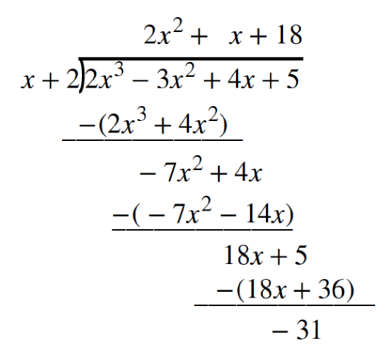
There is a lot of repetition in the table. If we don’t write the variables but, instead, line up their coefficients in columns under the division sign and also eliminate the partial products, we already have a simpler version of the entire problem.

$CNX_Precalc_Figure_03_05_004.jpg$

Synthetic division carries this simplification even a few more steps. Collapse the table by moving each of the rows up to fill any vacant spots. Also, instead of dividing by 2, as we would in division of whole numbers, then multiplying and subtracting the middle product, we change the sign of the “divisor” to –2, multiply and add. The process starts by bringing down the leading coefficient.

$CNX_Precalc_Figure_03_05_011.jpg$

We then multiply it by the “divisor” and add, repeating this process column by column, until there are no entries left. The bottom row represents the coefficients of the quotient; the last entry of the bottom row is the remainder. In this case, the quotient is $2x^2–7x+18$ and the remainder is –31.The process will be made more clear in Example $\PageIndex{3}$.

Synthetic Division

Synthetic division is a shortcut that can be used when the divisor is a binomial in the form $x−k$. In synthetic division, only the coefficients are used in the division process.

$how-to.png$ Given two polynomials, use synthetic division to divide

Write $k$ for the divisor.
Write the coefficients of the dividend.
Bring the lead coefficient down.
Multiply the lead coefficient by $k$. Write the product in the next column.
Add the terms of the second column.
Multiply the result by $k$. Write the product in the next column.
Repeat steps 5 and 6 for the remaining columns.
Use the bottom numbers to write the quotient. The number in the last column is the remainder and has degree 0, the next number from the right has degree 1, the next number from the right has degree 2, and so on.

Example $\PageIndex{3}$: Using Synthetic Division to Divide a Second-Degree Polynomial

Use synthetic division to divide $5x^2−3x−36$ by $x−3$.

Solution

Begin by setting up the synthetic division. Write $k$ and the coefficients.

$CNX_Precalc_Figure_03_05_005.jpg$

Bring down the lead coefficient. Multiply the lead coefficient by $k$.

$CNX_Precalc_Figure_03_05_006.jpg$

Continue by adding the numbers in the second column. Multiply the resulting number by $k$.Write the result in the next column. Then add the numbers in the third column.

$CNX_Precalc_Figure_03_05_007.jpg$

The result is $5x+12$. The remainder is 0. So $x−3$ is a factor of the original polynomial.

Analysis

Just as with long division, we can check our work by multiplying the quotient by the divisor and adding the remainder.

\[(x−3)(5x+12)+0=5x^2−3x−36\]

Example $\PageIndex{4}$: Using Synthetic Division to Divide a Third-Degree Polynomial

Use synthetic division to divide $4x^3+10x^2−6x−20$ by $x+2$.

Solution

The binomial divisor is $x+2$ so $k=−2$. Add each column, multiply the result by –2, and repeat until the last column is reached.

$CNX_Precalc_Figure_03_05_008.jpg$

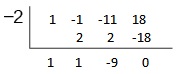
The result is $4x^2+2x−10$.

The remainder is 0. Thus, $x+2$ is a factor of $4x^3+10x^2−6x−20$.

Analysis

The graph of the polynomial function $f(x)=4x^3+10x^2−6x−20$ in Figure $\PageIndex{2}$ shows a zero at $x=k=−2$. This confirms that $x+2$ is a factor of $4x^3+10x^2−6x−20$.

Example $\PageIndex{5}$: Using Synthetic Division to Divide a Fourth-Degree Polynomial

Use synthetic division to divide $−9x^4+10x^3+7x^2−6$ by $x−1$.

Solution

Notice there is no x-term. We will use a zero as the coefficient for that term.

$CNX_Precalc_revised_eq_5.png$

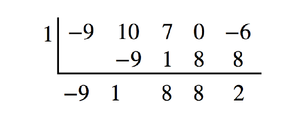
The result is $−9x^3+x^2+8x+8+\frac{2}{x−1}$.

$try-it.png$ $\PageIndex{5}$

Use synthetic division to divide $3x^4+18x^3−3x+40$ by $x+7$.

Solution: $3x^3−3x^2+21x−150+\frac{1,090}{x+7}$

Contributors

Jay Abramson (Arizona State University) with contributing authors. Textbook content produced by OpenStax College is licensed under a Creative Commons Attribution License 4.0 license. Download for free at https://openstax.org/details/books/precalculus.

Search

Text Color

Text Size

Margin Size

Font Type