3.5: Finding Information About Functions From Graphs

Learning Objectives

• Use a graph to find domain and range.
• Use a graph to determine where a function is increasing, decreasing, or constant.
• Use a graph to locate local maxima and local minima.
• Use a graphing calculator to describe behavior of functions.

Are You Ready?

Try these questions prior to beginning this section to help determine if you are set up for success:

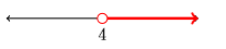
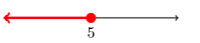
1. Use interval notation to describe the shaded region on the given number line.

   1. 

       

   2. 

       

       

Answer

1. 1. \((4, \infty)\)
   2. \((-\infty, 5]\)

If you missed this problem or feel you could use more practice, review [2.1: Real Numbers, Linear Inequalities, and Interval Notation]

We have been learning a lot about functions in this course. Understanding their unique features and how they behave is helpful when determining which functions will be the best models when describing real-life situations. In this section, we will focus on what information we can gain about functions from a graph.

Finding Domain and Range from Graphs

We have learned how to find the domain of functions algebraically. In many cases, find range algebraically is not so simple as there are no systematic approaches since the output behavior of functions can vary a lot depending on the equation of the functions. Another way to identify the domain and range of functions is by using graphs. Because the domain refers to the set of possible input values, the domain of a graph consists of all the input values shown on the x-axis. The range is the set of possible output values, which are shown on the y-axis. Keep in mind that if the graph continues beyond the portion of the graph we can see (as noted by arrows on the ends of the graph), the domain and range may be greater than the visible values shown in the coordinate system. See Figure \(\PageIndex{1}\).

Figure \(\PageIndex{1}\): Graph of a polynomial that shows the x-axis is the domain and the y-axis is the range

We can observe that the graph extends horizontally from −5 to the right without bound, so the domain is \(\left[−5,∞\right)\). The vertical extent of the graph is all range values 5 and below, so the range is \(\left(−∞,5\right]\). Note that the domain and range are always written from smaller to larger values, or from left to right for domain, and from the bottom of the graph to the top of the graph for range.

Example \(\PageIndex{1}\)

Find the domain and range of the function f whose graph is shown in Figure \(\PageIndex{2}\).

Figure \(\PageIndex{2}\): Graph of a function from (-3, 1].

Solution

We can observe that the horizontal extent of the graph is –3 to 1, so the domain of f is \(\left(−3,1\right]\).

The vertical extent of the graph is 0 to –4 and it appears there is a point at \((0,0)\) so the range is \(\left[−4,0\right]\). 

Example \(\PageIndex{2}\)

Find the domain and range of the function f whose graph is shown in Figure \(\PageIndex{3}\).

Figure \(\PageIndex{3}\): Graph of the Alaska Crude Oil Production where the y-axis is thousand barrels per day and the -axis is the years(credit: modification of work by the U.S. Energy Information Administration)

Solution

The input quantity along the horizontal axis is “years,” which we represent with the variable t for time. The output quantity is “thousands of barrels of oil per day,” which we represent with the variable b for barrels. The graph may continue to the left and right beyond what is viewed, but based on the portion of the graph that is visible, we can determine the domain as \(1973≤t≤2008\) and the range as approximately \(180≤b≤2010\).

In interval notation, the domain is \([1973, 2008]\), and the range is about \([180, 2010]\). For the domain and the range, we approximate the smallest and largest values since they do not fall exactly on the grid lines.

Using a Graphing Calculator to Find Domain and Range

We’ve learned how to find the domain and range of a function by looking at a graph. If we define a function by means of an equation, such as \(f(x)=\sqrt{4-x}\), then we should be able to capture the domain and range of f from its graph, provided, of course, that we can draw the graph of f. If we don't know what a graph looks like, we can use graphing technology.

Example \(\PageIndex{3}\)

Use a graphing calculator to estimate the domain and range using interval notation for the function defined by

\[f(x)=\sqrt{4-x}\nonumber\].

Solution

Load the expression defining f into the Y= menu, as shown in Figure \(\PageIndex{4}\)(a). Select 6:ZStandard from the ZOOM menu to produce the graph of f shown in Figure \(\PageIndex{5}\)(b).

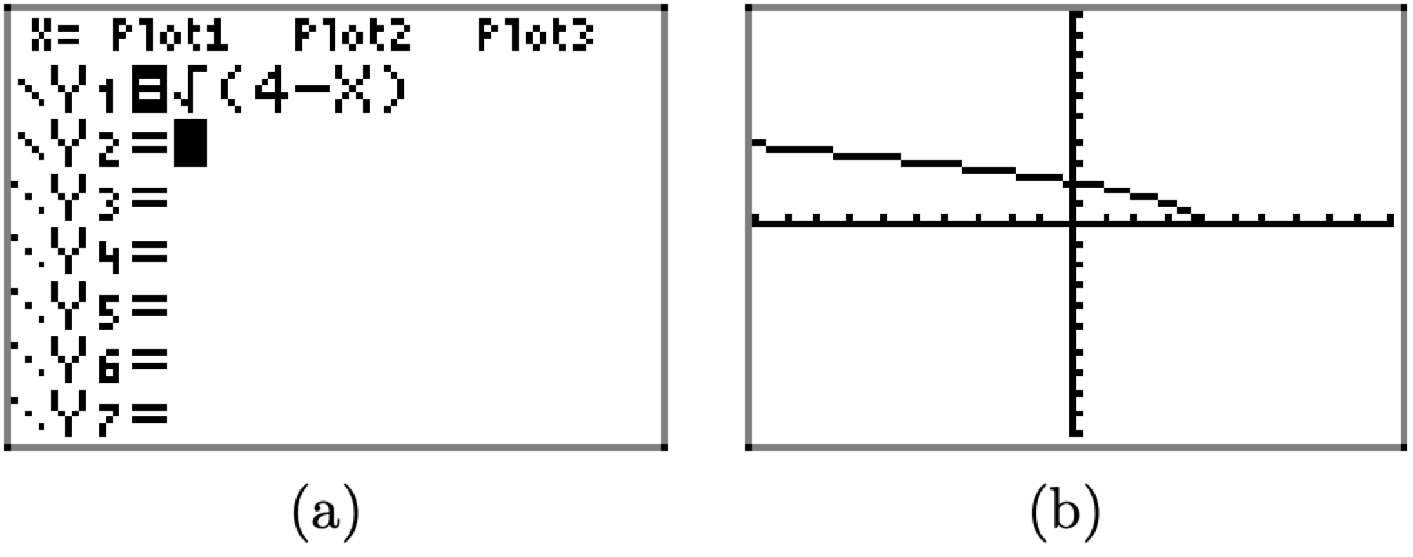
Figure \(\PageIndex{4}\). Sketching the graph of \(f(x)=\sqrt{4-x}\).

Next, project each point on the graph of f onto the x-axis, as shown in Figure \(\PageIndex{4}\)(b) to estimate the domain. Note that we’ve made two assumptions about the graph of f.

1. At the left end of the graph in Figure \(\PageIndex{4}\)(b), we assume that the graph of f continues upward and to the left indefinitely. Hence, the “shadow” or projection onto the x-axis will move indefinitely to the left. This is indicated by attaching an arrowhead to the left-hand end of the region that “lies in shadow” on the x-axis, as shown in Figure \(\PageIndex{4}\)(b).
2. We also assume that the right end of the graph ends at the point \((4, 0)\). This accounts for the “filled dot” when this point on the graph of f is projected onto the x-axis.

Note that the “shadow” or projection onto the x axis in Figure \(\PageIndex{4}\)(b) includes all values of x less than or equal to 4. Thus, the domain of f is \[\text { Domain of } f=(-\infty, 4]=\{x : x \leq 4\}\nonumber\]

We can also see this result by considering how f is defined.

\[f(x)=\sqrt{4-x}\nonumber\]

Recall that we earlier defined the domain of f as the set of “permissible” x-values. In this case, it is impossible to take the square root of a negative number, so we must be careful selecting the x-values we use in this rule. Note that \(x = 4\) is allowable, as

\[f(0)=\sqrt{4-4}=\sqrt{0}=0\nonumber\]

However, numbers larger than 4 cannot be used in this rule. For example, consider what happens when we attempt to use \(x = 5\).

\[f(x)=\sqrt{4-5}=\sqrt{-1}\nonumber\]

We’ll leave it to our readers to test other values of x that are less than 4. They will also produce real answers when they are input into the rule \(f(x)=\sqrt{4-x}\). Note that this also verifies our earlier conjecture that the “shadow” or projection shown in Figure \(\PageIndex{4}\)(b) continues indefinitely to the left.

Instead of “guessing and checking,” we can speed up the analysis of the domain of \(f(x)=\sqrt{4-x}\) by noting that the expression under the radical must not be a negative number. Hence, \(4 − x\) must either be greater than or equal to zero. This argument produces an inequality that is easily solved for x.

\[\begin{aligned} 4-x & \geq 0 \\-x & \geq-4 \\ x & \leq 4 \end{aligned}\]

This last result verifies that the domain of f is all values of x that are less than or equal to 4, which is in complete agreement with the “shadow” or projection onto the x-axis shown in Figure \(\PageIndex{4}\)(b).

Simliary, to determine the range of f, we project each point on the graph of f onto the y-axis. We estimate the range as

\[\text { Range of } f=[0, \infty)\nonumber\]

Using a Graph to Determine Where a Function is Increasing, Decreasing, or Constant

As part of exploring how functions change, we can identify intervals over which the function is changing in specific ways. We say that a function is increasing on an interval if the function values increase as the input values increase within that interval. Similarly, a function is decreasing on an interval if the function values decrease as the input values increase over that interval. Figure \(\PageIndex{5}\) shows examples of increasing and decreasing intervals on a function.

Figure \(\PageIndex{5}\): The function \(f(x)=x^3−12x\) is increasing on \((−\infty, −2)\cup (2,\infty)\) and is decreasing on \((−2, 2)\).

Increasing and Decreasing Function Behavior

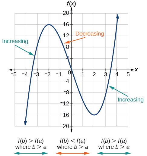
• A function \(f\) is increasing on an open interval if \(f(b)>f(a)\) for every \(a\), \(b\) within the interval where \(b>a\).
• A function \(f\) is decreasing on an open interval if \(f(b)<f(a)\) for every \(a\), \(b\) within interval where \(b>a\).
• A function \(f\) is constant on an open interval otherwise.

Increasing and Decreasing Behavior for Basic Functions

We will now return to our basic toolkit functions and discuss their graphical behavior in Figure \(\PageIndex{6}\). Note that this list includes some other functions that were not discussed in the previous section.

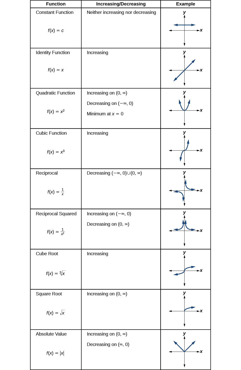
Figure \(\PageIndex{6}\)

Local Extrema

While some functions are increasing (or decreasing) over their entire domain, many are not. A continuous function is a function whose graph can be drawn in one movement without having to lift your pencil. If a function is continuous, a value of the input where a function changes from increasing to decreasing (as we go from left to right, that is, as the input variable increases) is called a local maximum. If a function has more than one, we say it has local maxima. Similarly, a value of the input where a function changes from decreasing to increasing as the input variable increases is called a local minimum. The plural form is “local minima.” Together, local maxima and minima are called local extrema of the function. Local extrema may are be referred to as relative extrema.

Clearly, a function is neither increasing nor decreasing on an interval where it is constant. A function is also neither increasing nor decreasing at extrema. Note that we have to speak of local extrema, because any given local extrema as defined here is not necessarily the highest maximum or lowest minimum in the function’s entire domain.

For the function whose graph is shown in Figure \(\PageIndex{7}\), the local maximum is 16, and it occurs at \(x=−2\). The local minimum is −16 and it occurs at \(x=2\).

Figure \(\PageIndex{7}\): Graph of a polynomial that shows the increasing and decreasing intervals and local maximum.maximum

To locate the local maxima and minima from a graph, we need to observe the graph to determine where the graph attains its highest and lowest points, respectively, within an open interval. Like the summit of a roller coaster, the graph of a function is higher at a local maximum than at nearby points on both sides. The graph will also be lower at a local minimum than at neighboring points. Figure \(\PageIndex{8}\) illustrates these ideas for a local maximum.

Figure \(\PageIndex{8}\): Definition of a local maximum

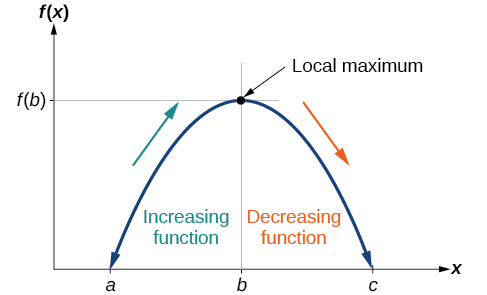
These observations lead us to a formal definition of local extrema.

Local Extrema

• A function \(f\) has a local maximum at a point \(b\) in an open interval \((a,c)\) if \(f(b)\) is greater than or equal to \(f(x)\) for every point \(x\) (\(x\) does not equal \(b\)) in the interval.
• A function \(f\) has a local minimum at a point \(b\) in \((a,c)\) if \(f(b)\) is less than or equal to \(f(x)\) for every \(x\) (\(x\) does not equal \(b\)) in the interval.

Example \(\PageIndex{4}\)

Given the function \(p(t)\) in Figure \(\PageIndex{9}\), identify the intervals on which the function appears to be increasing.

Figure \(\PageIndex{9}\): Graph of a polynomial.

Solution

We see that the function is not constant on any interval. The function is increasing where it slants upward as we move to the right and decreasing where it slants downward as we move to the right. The function appears to be increasing from \(t=1\) to \(t=3\) and from \(t=4\) on.

In interval notation, we would say the function appears to be increasing on the interval \((1,3)\) and the interval \((4,\infty)\).

Analysis

Notice in this example that we used open intervals (intervals that do not include the endpoints), because the function is neither increasing nor decreasing at \(t=1\), \(t=3\), and \(t=4\). These points are the local extrema (two minima and a maximum).

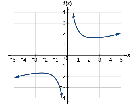
Example \(\PageIndex{5}\)

Graph the function \(f(x)=\frac{2}{x}+\frac{x}{3}\). Then use the graph to estimate the local extrema of the function and to determine the intervals on which the function is increasing.

Solution

Using technology, we find that the graph of the function looks like that in Figure \(\PageIndex{10}\). It appears there is a low point, or local minimum, between \(x=2\) and \(x=3\), and a mirror-image high point, or local maximum, somewhere between \(x=−3\) and \(x=−2\)

.

Figure \(\PageIndex{10}\): Graph of a rational function.

Analysis

Most graphing calculators and graphing utilities can estimate the location of maxima and minima. Figure \(\PageIndex{11}\) provides screen images from two different technologies, showing the estimate for the local maximum and minimum.

Figure \(\PageIndex{11}\): Graph of the reciprocal function on a graphing calculator.

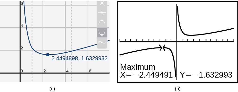
Based on these estimates, the function is increasing on the interval \((−\infty,−2.449)\) and \((2.449,\infty)\). Notice that, while we expect the extrema to be symmetric, the two different technologies agree only up to four decimals due to the differing approximation algorithms used by each. (The exact location of the extrema is at \(\pm\sqrt{6}\), but determining this requires calculus.)

You Try \(\PageIndex{1}\)

Graph the function \(f(x)=x^3−6x^2−15x+20\) in a graphing calculator to estimate the local extrema of the function. Use these to determine the intervals on which the function is increasing and decreasing.

Solution

The local maximum appears to occur at \((−1,28)\), and the local minimum occurs at \((5,−80)\). The function is increasing on \((−\infty,−1)\cup(5,\infty)\) and decreasing on \((−1,5)\).

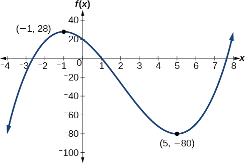
Graph of a polynomial with a local maximum at (-1, 28) and local minimum at (5, -80).

Example \(\PageIndex{6}\)

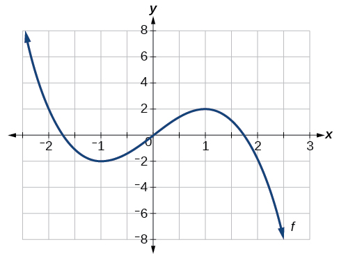
For the function f whose graph is shown in Figure \(\PageIndex{12}\), find all local maxima and minima.

Figure \(\PageIndex{12}\): Graph of a polynomial.

Solution

Observe the graph of \(f\). The graph attains a local maximum at \(x=1\) because it is the highest point in an open interval around \(x=1\).The local maximum is the y-coordinate at \(x=1\), which is 2.

The graph attains a local minimum at \(x=−1\) because it is the lowest point in an open interval around \(x=−1\). The local minimum is the y-coordinate at \(x=−1\), which is −2.

Contributors and Attributions

• Jay Abramson (Arizona State University) with contributing authors. Textbook content produced by OpenStax College is licensed under a Creative Commons Attribution License 4.0 license. Download for free at https://openstax.org/details/books/precalculus.