4.3: Graphs of Polynomial Functions

Learning Objectives

• Identify polynomial functions.
• Identify end behavior of polynomial functions.
• Find x-intercepts of polynomial functions.

Are You Ready?

Try these questions prior to beginning this section to help determine if you are set up for success:

1. Identify the degree and leading coefficient of the given polynomial: \(4x^3-7x^5+9x^4-11+2x-x^4\)
2. Solve:
   1. \(\quad 2j^3-3j^2=8j-12\)
   2. \(\quad 4c^2=12c\)

Answer

1. The degree is 5 and the leading coefficient is -7

If you missed this problem or feel you could use more practice, review [2.3: Polynomial Expressions]

2. 1. \(\quad j=-2\text{, }\dfrac{3}{2}\text{, }2\)
   2. \(\quad c=0\text{, }3\)

If you missed this problem or feel you could use more practice, review [2.8: Solving Polynomial Equations, 2.24: Solving Quadratic Equations Using the Square Root Property, 2.25: Solving Quadratic Equations by Completing the Square, and 2.26: Solving Quadratic Equations Using the Quadratic Formula]

Polynomial functions are used widely for modeling many real-life situations. In this section, we will investigate the common traits of this important family of functions.

Polynomial Function

A polynomial function is a function of the form

\[ f(x) = a_{n} x^{n} + a_{n-1}x^{n-1} + \ldots + a_{2}x^{2} + a_{1}x + a_0, \label{polynomialfunction}\nonumber \]

where \(a_0\), \(a_1\), ... , \(a_{n}\) are real numbers and \(n \geq 1\) is a natural number. The domain of a polynomial function is \((-\infty, \infty)\).

• The natural number \(n\) is called the degree of the polynomial \(f\).
• The term \(a_{n} x^{n}\) is called the leading term of the polynomial \(f\).
• The real number \(a_{n}\) is called the leading coefficient of the polynomial \(f\).
• The real number \(a_{0}\) is called the constant term of the polynomial \(f\).

Example \(\PageIndex{1}\)

Determine if the following functions are polynomials. If they are, identify the degree, leading term, leading coefficient and constant term.

1. \(f(x) = 4x^5 - 3x^2 + 2x - 5\)
2. \(g(x) = 12x - x^3\)
3. \(p(x) = \dfrac{4x+x^3}{x}\)
4. \(h(x) = \dfrac{4-x}{5}\)
5. \(A(x) = (2x-1)^{3}(x-2)(3x+2)\)

Solution

1. This is a polynomial function by definition, and we see that the degree is \(5\), the leading term is \(4x^5\), the leading coefficient is \(4\) and the constant term is \(-5\).
2. The definition of a polynomial function has the highest power of \(x\) first. To that end, we re-write \(g(x) = 12x - x^3 =-x^3+12x\), and see that the degree of \(g\) is \(3\), the leading term is \(-x^3\), the leading coefficient is \(-1\) and the constant term is \(0\).
3. Even though \(p(x) = \dfrac{x^3+4x}{x}\) simplifies to \(p(x) = x^2+4\), which certainly looks like a polynomial function, the domain of \(p\) excludes \(0\). Alas, \(p\) is not a polynomial function.
4. \(h\) can be rewritten as follows: \(h(x) = \dfrac{4-x}{5} = \dfrac{4}{5} - \dfrac{x}{5} = -\dfrac{1}{5} x + \dfrac{4}{5}\). The degree of \(h\) is \(1\), the leading term is \(-\dfrac{1}{5} x\), the leading coefficient is \(-\dfrac{1}{5}\) and the constant term is \(\dfrac{4}{5}\).
5. It may seem that we have some work ahead of us to get \(A\) in the form provided in the definition of a polynomial function. However, it is possible to gain the information requested about \(A\) without multiplying out the entire expression \((2x-1)^{3}(x-2)(3x+2)\). The leading term of \(A\) will be the term which has the highest power of \(x\). The way to get this term is to multiply the terms with the highest power of \(x\) from each factor together - in other words, the leading term of \(A(x)\) is the product of the leading terms of the factors of \(A(x)\). Hence, the leading term of \(A\) is \((2x)^3(x)(3x) = 24x^5\). This means that the degree of \(A\) is \(5\) and the leading coefficient is \(24\). As for the constant term, we can perform a similar trick. The constant term is obtained by multiplying the constant terms from each of the factors \((-1)^3(-2)(2) = 4\).

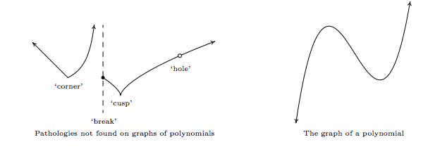
Now that we know how to identify polynomial functions, we can start to investigate their graphical behavior. Polynomial functions share two properties which help distinguish them from other animals (functions) in the algebra zoo: they are continuous and smooth. While these concepts are formally defined in Calculus, informally, polynomial graphs have no 'breaks', 'holes', or 'sharp turns' (also known as a 'cusp'). Below, in Figure \(\PageIndex{1}\), on the left we a graph of a function which is neither smooth nor continuous, and to its right we have a graph of a polynomial, for comparison.

Figure \(\PageIndex{1}\): Graph of a function that is not a polynomial and a graph of a polynomial.

Next, let's look at monomials (single term polynomials) to help us establish some graphical pattern that is similar with all polynomials.

End Behavior of Polynomial Functions

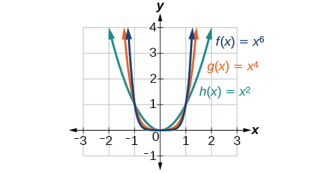
Figure \(\PageIndex{2}\) shows the graphs of \(f(x)=x^2\), \(g(x)=x^4\) and and \(h(x)=x^6\), which are monomial functions with even degrees. Notice that these graphs have similar shapes, very much like that of the basic quadratic function. They are commonly called basic even-power functions. However, as the power increases, the graphs flattens near the origin within the interval \((-1,1)\) and becomes steeper must faster outside of this interval.

Figure \(\PageIndex{2}\): Even-power functions

To describe the behavior as numbers become larger and larger, we use the idea of infinity. We use the symbol \(\infty\) for positive infinity and \(−\infty\) for negative infinity. When we say that “x approaches infinity,” which can be symbolically written as \(x{\rightarrow}\infty\), we are describing a behavior; we are saying that \(x\) is increasing without bound.

With the even-degree monomial functions, as the input increases or decreases without bound, the output values become very large, positive numbers. Equivalently, we could describe this behavior by saying that as \(x\) approaches positive or negative infinity, the \(f(x)\) values increase without bound. In symbolic form, we write this as

\[\text{as } x{\rightarrow}{\pm}{\infty}, \;f(x){\rightarrow}{\infty} \nonumber \]

Figure \(\PageIndex{3}\) shows the graphs of \(f(x)=x^3\), \(g(x)=x^5\), and \(h(x)=x^7\), which are all odd degree monomial functions, commonly called basic odd-degree power functions. Notice that these graphs look similar to the basic cubic function in the toolkit. Again, as the power increases, the graphs flatten near the origin and become steeper away from the origin.

Figure \(\PageIndex{3}\): Odd-power function

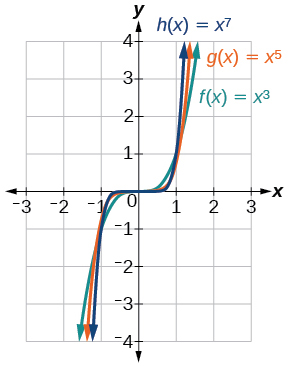
These examples illustrate that functions of the form \(f(x)=x^n\) where \(n\) is a positive integer reveal symmetry of one kind or another. First, in Figure \(\PageIndex{2}\) we see that functions of the form \(f(x)=x^n\), \(n\) even, are symmetric about the \(y\)-axis. In Figure \(\PageIndex{3}\) we see that functions of the form \(f(x)=x^n\), \(n\) odd, are symmetric about the origin.

For these odd powered functions, as \(x\) approaches negative infinity, \(f(x)\) decreases without bound. As \(x\) approaches positive infinity, \(f(x)\) increases without bound. In symbolic form we write

\[\begin{align*} &\text{as }x{\rightarrow}-{\infty},\;f(x){\rightarrow}-{\infty} \\ &\text{as }x{\rightarrow}{\infty},\;f(x){\rightarrow}{\infty} \end{align*}\nonumber \]

The behavior of the graph of a function as the input values get very small \((x{\rightarrow}−{\infty})\) and get very large \(x{\rightarrow}{\infty}\) is referred to as the end behavior of the function. We can use words or symbols to describe end behavior.

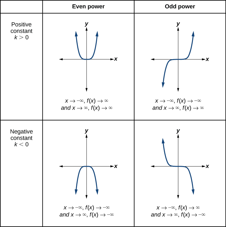
Figure \(\PageIndex{4}\) shows the end behavior of various monomial functions in the form \(f(x)=kx^n\) where \(n\) is a non-negative integer depending on the power and the constant.

Figure \(\PageIndex{4}\)

The end behavior describes above can be generalized for all polynomials as follows:

End Behavior of Even Degree Polynomial Functions

Suppose \(f(x) = a x^{n}\) where \(a \neq 0\) is a real number and \(n\) is an even natural number. The end behavior of the graph of \(y=f(x)\) matches one of the following:

• for \(a > 0\), as \(x \rightarrow -\infty\), \(f(x) \rightarrow \infty\) and as \(x \rightarrow \infty\), \(f(x) \rightarrow \infty\)
• for \(a < 0\), as \(x \rightarrow -\infty\), \(f(x) \rightarrow -\infty\) and as \(x \rightarrow \infty\), \(f(x) \rightarrow -\infty\)

Graphically:

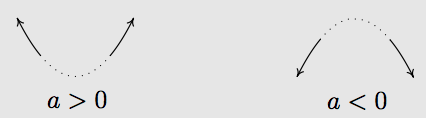
Figure \(\PageIndex{5}\)

End Behavior of Odd Degree Polynomial Functions

Suppose \(f(x) = a x^{n}\) where \(a \neq 0\) is a real number and \(n \geq 3\) is an odd natural number. The end behavior of the graph of \(y=f(x)\) matches one of the following:

1. for \(a > 0\), as \(x \rightarrow -\infty\), \(f(x) \rightarrow -\infty\) and as \(x \rightarrow \infty\), \(f(x) \rightarrow \infty\)
2. for \(a < 0\), as \(x \rightarrow -\infty\), \(f(x) \rightarrow \infty\) and as \(x \rightarrow \infty\), \(f(x) \rightarrow -\infty\)

Graphically:

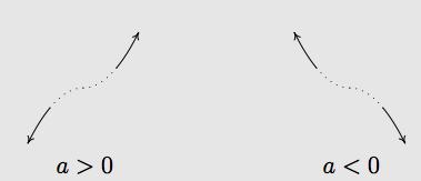
Figure \(\PageIndex{6}\)

Example \(\PageIndex{2}\)

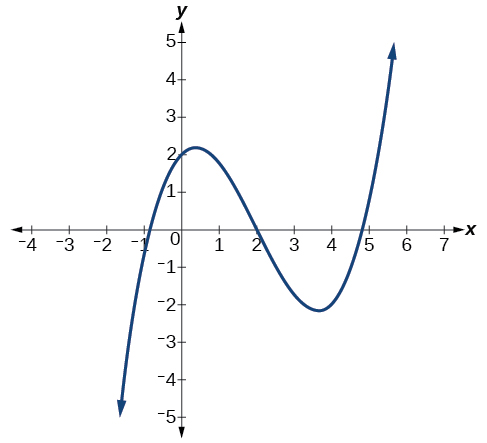
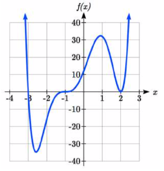
Describe the end behavior and determine a possible degree of the polynomial function in Figure \(\PageIndex{7}\).

Figure \(\PageIndex{7}\).

Solution

As the input values \(x\) get very large, the output values \(f(x)\) increase without bound. As the input values \(x\) get very small, the output values \(f(x)\) decrease without bound. We can describe the end behavior symbolically by writing

\[\text{as } x{\rightarrow}{\infty}, \; f(x){\rightarrow}{\infty} \nonumber \]

\[\text{as } x{\rightarrow}-{\infty}, \; f(x){\rightarrow}-{\infty} \nonumber \]

In words, we could say that as \(x\) values approach infinity, the function values approach infinity, and as \(x\) values approach negative infinity, the function values approach negative infinity.

We can tell this graph has the shape of an odd degree polynomial that has not been reflected, so the degree of the polynomial creating this graph must be odd and the leading coefficient must be positive.

You Try \(\PageIndex{1}\)

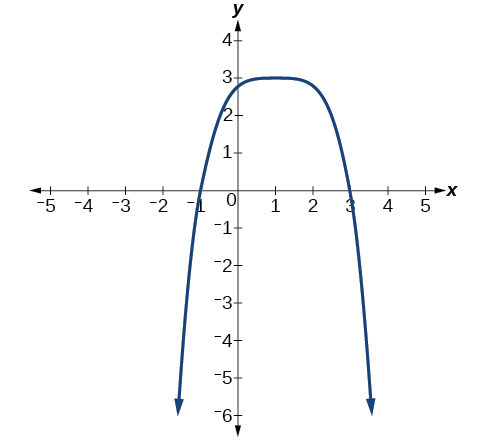
Describe the end behavior, and determine a possible degree of the polynomial function in Figure \(\PageIndex{8}\).

Figure \(\PageIndex{8}\)

Answer

As \(x{\rightarrow}{\infty}\), \(f(x){\rightarrow}−{\infty}\); as \(x{\rightarrow}−{\infty}\), \(f(x){\rightarrow}−{\infty}\). It has the shape of an even degree polynomial function with a negative coefficient.

Example \(\PageIndex{3}\)

Given the function \(f(x)=−3x^2(x−1)(x+4)\), determine the leading term, degree, and end behavior of the function.

Solution

First, expand the function,

\[\begin{align*} f(x)&=−3x^2(x−1)(x+4) \\ &=−3x^2(x^2+3x−4) \\ &=−3x^4−9x^3+12x^2 \end{align*}\]

The leading term is \(−3x^4\); therefore, the degree of the polynomial is 4. The degree is even (4) and the leading coefficient is negative (–3), so the end behavior is

\[\text{as }x{\rightarrow}−{\infty}, \; f(x){\rightarrow}−{\infty} \nonumber \]

\[\text{as } x{\rightarrow}{\infty}, \; f(x){\rightarrow}−{\infty} \nonumber \]

You Try \(\PageIndex{2}\)

Given the function \(f(x)=0.2(x−2)(x+1)(x−5)\), determine the leading term, degree, and end behavior of the function.

Answer

The leading term is \(0.2x^3\), so it is a degree 3 polynomial.

\[\text{as }x{\rightarrow}−{\infty}, \; f(x){\rightarrow}−{\infty} \nonumber \]

\[\text{as } x{\rightarrow}{\infty}, \; f(x){\rightarrow}{\infty} \nonumber \]

Identifying Local Behavior of Polynomial Functions

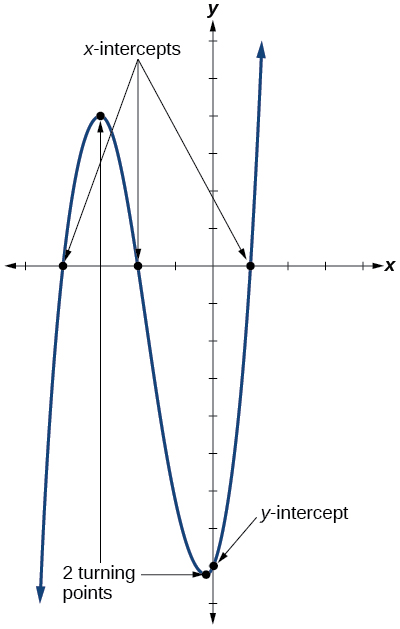
In addition to the end behavior of polynomial functions, we are also interested in what happens in the “middle” of the function. In particular, we are interested in the intercepts and turning points. As with all functions, the \(y\)-intercept is the point at which the graph intersects the vertical axis. The point corresponds to the coordinate pair in which the input value is zero. Because a polynomial is a function, only one output value corresponds to each input value so there can be only one \(y\)-intercept \((0,a_0)\). The \(x\)-intercepts occur at the input values that correspond to an output value of zero. It is possible to have more than one \(x\)-intercept. See Figure \(\PageIndex{9}\). Turning points are local extrema values. We may approximate them using technology but it will take calculus to find them exactly. Hence, we will focus our time in this course are finding intercepts only.

Figure \(\PageIndex{9}\)

Before we look at finding intercepts, let's note some important theory about graphical behavior.

The Intermediate Value Theorem

Suppose \(f\) is a continuous function on an interval containing \(x=a\) and \(x=b\) with \(a<b\). If \(f(a)\) and \(f(b)\) have different signs, then \(f\) has at least one zero between \(x = a\) and \(x = b\); that is, for at least one real number \(c\) such that \(a < c < b\), we have \(f(c) = 0\).

The Intermediate Value Theorem is extremely profound; it gets to the heart of what it means to be a real number, and is one of the most often used and under appreciated theorems in Mathematics. With that being said, most students see the result as common sense since it says, geometrically, that the graph of a polynomial function cannot be above the \(x\)-axis at one point and below the \(x\)-axis at another point without crossing the \(x\)-axis somewhere in between.

Example \(\PageIndex{4}\)

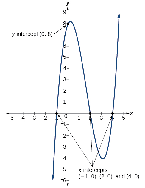
Given the polynomial function \(f(x)=(x−2)(x+1)(x−4)\), determine the \(y\)- and \(x\)-intercepts.

Solution

The \(y\)-intercept occurs when the input is zero, so substitute 0 for \(x\).

\[ \begin{align*}f(0)&=(0−2)(0+1)(0−4) \\ &=(−2)(1)(−4) \\ &=8 \end{align*} \nonumber \]

The \(y\)-intercept is \((0,8)\).

The \(x\)-intercepts occur when the output is zero. The function is already factored which makes this equation very nice to solve:

\[ 0=(x−2)(x+1)(x−4) \nonumber \]

\[\begin{array}{l} {x-2 =0} \\ {x=2} \end{array} \qquad \text{ or } \qquad \begin{array}{l} {x+1=0} \\ {x =-1} \end{array}\qquad \text{ or } \qquad \begin{array}{l} {x-4 =0} \\ {x =4} \end{array} \nonumber \]

The \(x\)-intercepts are \((2,0)\),\((–1,0)\), and \((4,0)\).

We can see these intercepts on the graph of the function shown in Figure \(\PageIndex{10}\).

Figure \(\PageIndex{10}\): Graph of \(f(x)=(x-2)(x+1)(x-4)\).

You Try \(\PageIndex{3}\)

Given the polynomial function \(f(x)=2x^3−6x^2−20x\), determine the intercepts.

Answer

\(x\)-intercepts \((0,0)\),\((–2,0)\), and \((5,0)\), \(y\)-intercept \((0,0)\);

Example \(\PageIndex{5}\)

Find the x-intercepts of \(f(x)=x^{6} -3x^{4} +2x^{2}\).

Solution

We can attempt to factor this polynomial to find solutions for \(f(x) = 0\).

\[x^{6} -3x^{4} +2x^{2} =0 \nonumber\] Factoring out the greatest common factor

\[x^{2} (x^{4} -3x^{2} +2)=0 \nonumber \] Factoring the inside as a quadratic in x\({}^{2}\)

\[x^{2} (x^{2} -1)(x^{2} -2)=0 \nonumber \] Then break apart to find solutions

\[\begin{array}{l} {x^{2} =0} \\[4pt] {x=0} \end{array}\qquad\text{ or } \qquad \begin{array}{l} {x^{2} -1=0} \\[4pt] {x^{2} =1} \\[4pt] {x=\pm 1} \end{array}\qquad \text{ or } \qquad \begin{array}{l} {x^{2} -2=0} \\[4pt] {x^{2} =2} \\ {x=\pm \sqrt{2} } \end{array} \nonumber \]

This gives us 5 x-intercepts: \((0,0)\), \((-\sqrt{2},0)\), \((–1,0)\), \((1,0)\), and \((\sqrt{2},0)\).

Example \(\PageIndex{6}\)

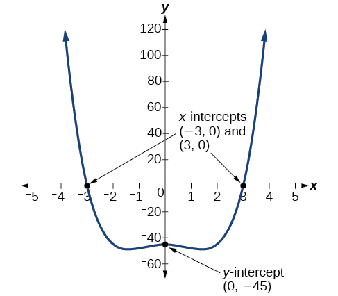
Given the polynomial function \(f(x)=x^4−4x^2−45\), determine the \(y\)- and \(x\)-intercepts.

Solution

The \(y\)-intercept occurs when the input is zero.

\[ \begin{align*} f(0) &=(0)^4−4(0)^2−45 \\[4pt] &=−45 \end{align*}\]

The \(y\)-intercept is \((0,−45)\).

The \(x\)-intercepts occur when the output is zero. To determine when the output is zero, we will need to factor the polynomial.

\[\begin{align*} f(x)&=x^4−4x^2−45 \\ &=(x^2−9)(x^2+5) \\ &=(x−3)(x+3)(x^2+5)
\end{align*}\]

\[0=(x−3)(x+3)(x^2+5) \nonumber \]

\[\begin{array}{l} {x-3 =0} \\ {x=3} \end{array} \qquad \text{ or } \qquad \begin{array}{l} {x+3=0} \\ {x =-3} \end{array}\qquad \text{ or } \qquad \begin{array}{l} {x^2+5=0} \\ \text{no real solution} \end{array} \nonumber \]

The \(x\)-intercepts are \((3,0)\) and \((–3,0)\).

We can see these intercepts on the graph of the function shown in Figure \(\PageIndex{11}\). We can see that the function is even because \(f(x)=f(−x)\).

Figure \(\PageIndex{11}\): Graph of \(f(x)=x^4-4x^2-45\).

Example \(\PageIndex{7}\)

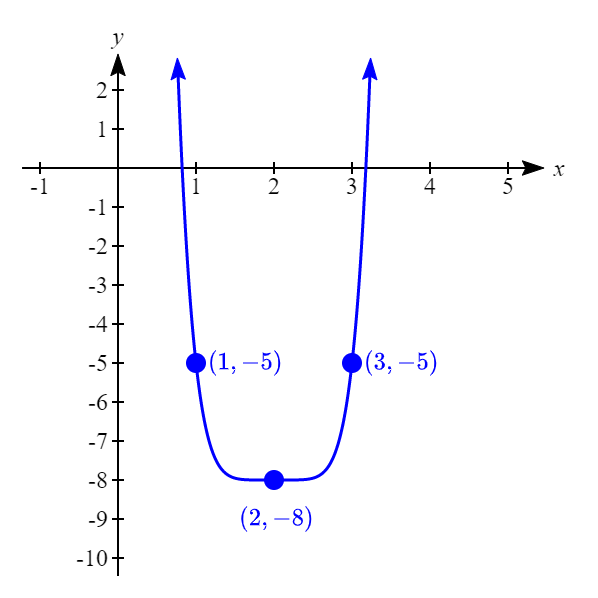
Find the intercepts of \(D(x)=3(x-2)^6-8\).

Solution

This is a basic even-power function that has has a horizontal shift right 2 units, vertical shift down 8 units, and a vertical stretch by 3. Since the basic shape is similar to a quadratic function, we know the graph opens up so that indicates that there are two x-intercepts. If you take a moment to sketch the function on graph paper using your knowledge of transformations, you will also notice that the x-intercepts should have x-coordinates close to 1 and 3. See Figure \(\PageIndex{12}\)

Figure \(\PageIndex{12}\): Graph of D(x)

Finding the x-intercepts, \[\begin{align*} 0&=3(x-2)^6-8\\[4pt] 8&=3(x-2)^6\\[4pt] \dfrac{8}{3}&=(x-2)^6\\[4pt] \pm\sqrt[6]{\dfrac{8}{3}}&=\sqrt[6]{(x-2)^6}\\[4pt] \pm\sqrt[6]{\dfrac{8}{3}}&=x-2\\[4pt] 2\pm\sqrt[6]{\dfrac{8}{3}}&=x\\[4pt] \end{align*}\]The x-intercepts are \(\left(2-\sqrt[6]{\dfrac{8}{3}},0\right)\) and \(\left(2+\sqrt[6]{\dfrac{8}{3}},0\right)\).

Note that if you approximate the x-intercepts that they should be about where we anticipated them to be when we sketched the graph.

Finding the y-intercept, \[\begin{align*} D(0)&=3(x-2)^6-8\\[4pt]&=3(0-2)^6-8\\[4pt]&=3(-2)^6-8\\[4pt]&=3(64)-8\\[4pt]&=184 \end{align*}\]The y-intercept is \((0,184)\).

Local Extrema of Polynomials

Recall that local extrema are function occur where a function changes from increasing to decreasing or from decreasing to increasing. Turning points for a graph of a polynomial function occur at extrema values. Although calculus is required to prove the following, this is an important theorem to know about the number of local extrema values we can expect for a polynomial function.

Number of Local Extrema for Polynomials

A polynomial of degree \(n\) will have at most \(n-1\) local extrema.

Note that a polynomial of degree \(n\) can have less than \(n-1\) local extrema. For example, \(P(x)=2x^5\) is a polynomial of degree 5 but it has no local extrema.

Graphical Behavior Near X-Intercepts

If we graph the function \(f(x)=(x+3)(x-2)^{2} (x+1)^{3}\), as shown in Figure \(\PageIndex{13}\), notice that the behavior at each of the x-intercepts is different.

Figure \(\PageIndex{13}\): Graph of \(f(x)=(x+3)(x-2)^{2} (x+1)^{3}\)

At the x-intercept at \((-3,0)\), which came from the \((x+3)\) factor of the polynomial, the graph passes directly through this horizontal intercept.

The factor \((x+3)\) is linear (has a power of 1), so the behavior near the intercept is like that of a line - it passes directly through the intercept. We call this a single zero, since the zero corresponds to a single factor of the function.

At the x-intercept at \((2,0)\), which came from the \((x-2)^{2}\) factor of the polynomial, the graph touches the axis at the intercept and then the graph bounces. The factor is quadratic (degree 2), so the behavior near the intercept is like that of a quadratic – it bounces off the horizontal axis at the intercept. Since \((x-2)^{2} =(x-2)(x-2)\), the factor is repeated twice, so we call this a double zero. We could also say the zero has multiplicity 2.

At the x-intercept at \((-1,0)\), which came from the \((x+1)^{3}\) factor of the polynomial, the graph passes through the axis at the intercept, but flattens out a bit first. This factor is cubic (degree 3), so the behavior near the intercept is like that of a cubic, with the same “S” type shape near the intercept that the cubic parent function, \(x^{3}\), has. We call this a triple zero. We could also say the zero has multiplicity 3.

By utilizing these behaviors, we can sketch a reasonable graph of a factored polynomial function without needing technology.

Graphical Behavior of Polynomials at X-intercepts

If a polynomial contains a factor of the form \((x-h)^{p}\), the behavior near the horizontal intercept \(h\) is determined by the power on the factor.

Figure \(\PageIndex{14}\): Graphical behavior of roots with various roots of multiplicities

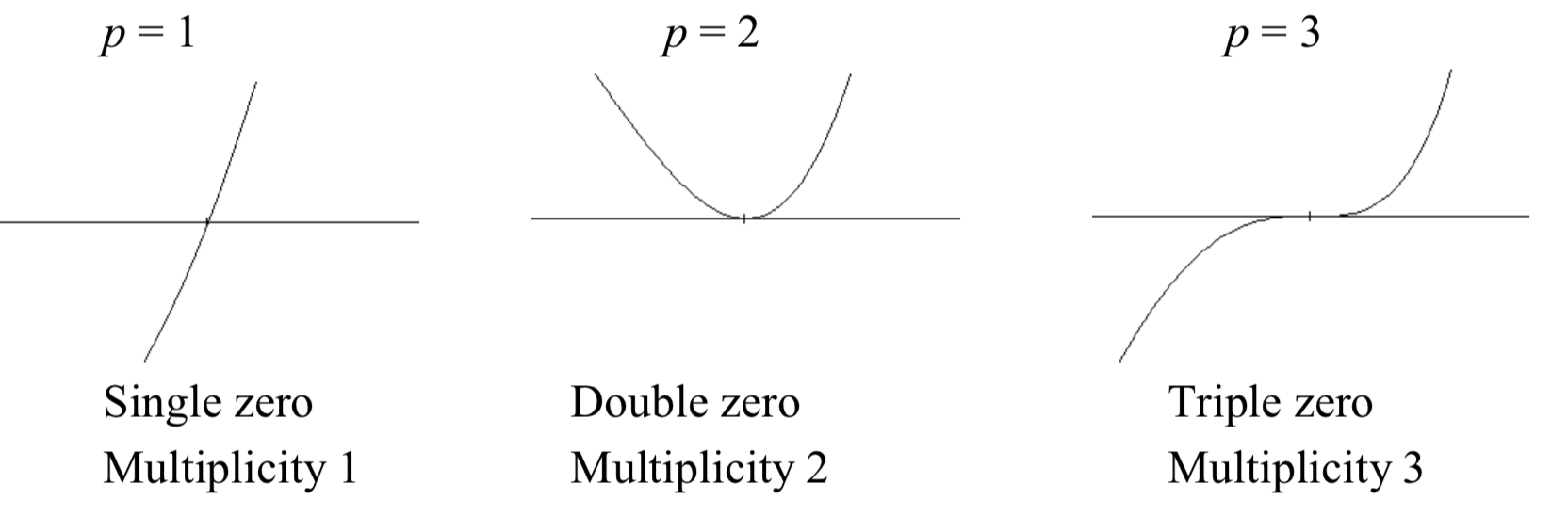
For higher even powers 4,6,8 etc.… the graph will bounce off the horizontal axis but the graph will appear flatter with each increasing even power as it approaches and leaves the axis.

For higher odd powers, 5,7,9 etc… the graph will pass through the horizontal axis but the graph will appear flatter with each increasing odd power as it approaches and leaves the axis.

Example \(\PageIndex{8}\)

Sketch a graph of \(f(x)=-2(x+3)^{2} (x-5)\).

Solution

This graph has two horizontal intercepts. At -3, the factor it came from is squared, indicating the graph will bounce at this horizontal intercept. At 5, the factor t came from is linear, indicating the graph will pass through the axis at this intercept.

Additionally, we can see the leading term, if this polynomial were multiplied out, would be \(-2x^{3}\), so the long-run behavior the left side of the graph will go upward and the right side will go downward.

To sketch this we consider the following:

Figure \(\PageIndex{15}\): Copy and Paste Caption here. (Copyright; author via source)

As \(x \to -\infty\) the function \(f(x) \to \infty\) so we know the graph starts in the 2\({}^{nd}\) quadrant and is decreasing toward the horizontal axis.

At (-3, 0) the graph bounces off the horizontal axis and so the function must start increasing.

At (0, 90) the graph crosses the vertical axis at the vertical intercept.

Somewhere after this point, the graph must turn back down or start decreasing toward the horizontal axis since the graph passes through the next intercept at (5,0).

As \(x \to \infty\) the function\(f(x) \to -\infty\) so we know the graph continues to decrease and we can stop drawing the graph in the 4\({}^{th}\) quadrant.

Using technology and an appropriate viewing window we can verify the shape of the graph.

Example \(\PageIndex{9}\)

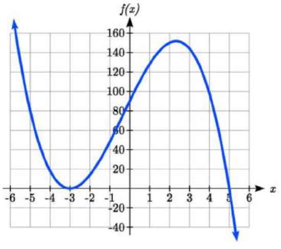
Write a formula for the polynomial function graphed in Figure \(PageIndex{16}\).

Figure \(\PageIndex{16}\): Graph of a polynomial with x-intercepts at (-3,0), (2,0), and (5,0)

Solution

This graph has three horizontal intercepts: \(x\) = -3, 2, and 5. At \(x\) = -3 and 5 the graph passes through the axis, suggesting the corresponding factors of the polynomial will be linear. At \(x = 2\) the graph bounces at the intercept, suggesting the corresponding factor of the polynomial will be 2\({}^{nd}\) degree (quadratic).

Together, this gives us:

\[f(x)=a(x+3)(x-2)^{2} (x-5) \nonumber\]

To determine the stretch factor, we can utilize another point on the graph. Here, the vertical intercept appears to be (0,-2), so we can plug in those values to solve for \(a\):

\[\begin{array}{l} {-2=a(0+3)(0-2)^{2} (0-5)} \\ {-2=-60a} \\ {a=\dfrac{1}{30} } \end{array} \nonumber\]

The graphed polynomial appears to represent the function

\[f(x)=\dfrac{1}{30} (x+3)(x-2)^{2} (x-5) \nonumber \]

You Try \(\PageIndex{4}\)

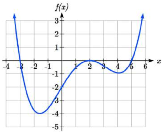
Given the graph, write a formula for the function shown in Figure \(\PageIndex{17}\).

Figure \(\PageIndex{17}\): Graph of a polynomial with x-intercepts at (-1,0), (2,0), and (4,0)

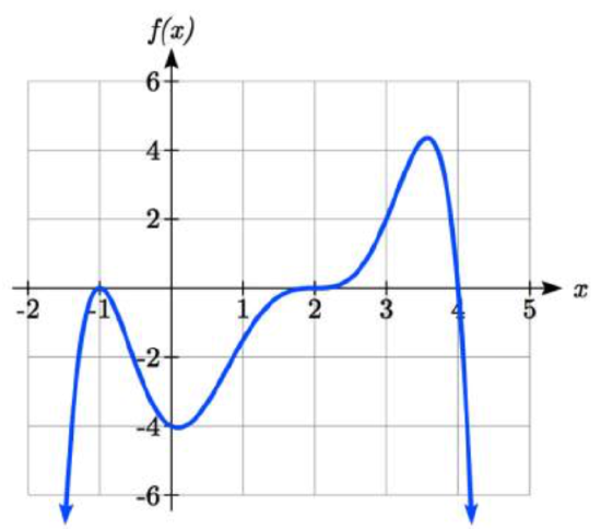
Answer

Double zero at \(x= - 1\), triple zero at \(x = 2\). Single zero at \(x = 4\). \(f(x) = a(x - 2)^{3} (x+1)^{2} (x-4)\). Substituting (0,-4) and solving for \(a\), \(f(x) = -\dfrac{1}{8} (x-2)^{3} (x+1)^{2} (x-4)\)

Let's look at a couple more examples to apply all that we have been learning.

Example \(\PageIndex{10}\)

A box with no top, also called a tray, is to be fashioned from a \(10\) inch \(\times\) \(12\) inch piece of cardboard by cutting out congruent squares from each corner of the cardboard and then folding the resulting tabs. Let \(x\) denote the length of the side of the square which is removed from each corner.

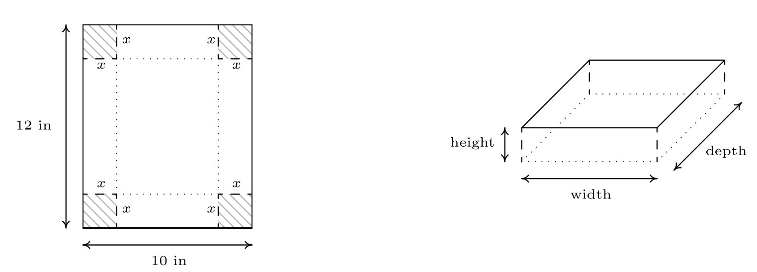
Find the volume \(V\) of the box as a function of \(x\). Include an appropriate applied domain.

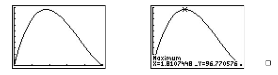
Use a graphing calculator to graph \(y=V(x)\) on the domain you found in part 1 and approximate the dimensions of the box with maximum volume to two decimal places. What is the maximum volume?

Solution

1. From Geometry, we know that \(\mbox{Volume} = \mbox{width} \times \mbox{height} \times \mbox{depth}\). The key is to find each of these quantities in terms of \(x\). From the figure, we see that the height of the box is \(x\) itself. The cardboard piece is initially \(10\) inches wide. Removing squares with a side length of \(x\) inches from each corner leaves \(10-2x\) inches for the width.\footnote{There's no harm in taking an extra step here and making sure this makes sense. If we chopped out a \(1\) inch square from each side, then the width would be \(8\) inches, so chopping out \(x\) inches would leave \(10-2x\) inches.} As for the depth, the cardboard is initially \(12\) inches long, so after cutting out \(x\) inches from each side, we would have \(12-2x\) inches remaining. As a function\footnote{When we write \(V(x)\), it is in the context of function notation, not the volume \(V\) times the quantity \(x\).} of \(x\), the volume is \[V(x) = x(10-2x)(12-2x) = 4x^3-44x^2+120x \nonumber \] To find a suitable applied domain, we note that to make a box at all we need \(x > 0\). Also the shorter of the two dimensions of the cardboard is \(10\) inches, and since we are removing \(2x\) inches from this dimension, we also require \(10 - 2x > 0\) or \(x < 5\). Hence, our applied domain is \(0 < x < 5\).

2. Using a graphing calculator, we see that the graph of \(y=V(x)\) has a relative maximum. For \(0 < x < 5\), this is also the absolute maximum. Using the 'Maximum' feature of the calculator, we get \(x \approx 1.81\), \(y \approx 96.77\). This yields a height of \(x \approx 1.81\) inches, a width of \(10 - 2x \approx 6.38\) inches, and a depth of \(12 - 2x \approx 8.38\) inches. The \(y\)-coordinate is the maximum volume, which is approximately \(96.77\) cubic inches (also written \(\mbox{in}^3\)).

In order to solve, we made good use of the graph of the polynomial \(y=V(x)\), so we ought to turn our attention to graphs of polynomials in general. Below are the graphs of \(y=x^2\), \(y=x^4\) and \(y=x^6\), side-by-side. We have omitted the axes to allow you to see that as the exponent increases, the 'bottom' becomes 'flatter' and the 'sides' become 'steeper.' If you take the the time to graph these functions by hand,\footnote{Make sure you choose some \(x\)-values between \(-1\) and \(1\).} you will see why.

We learned earlier in this course how to solve non-linear inequalities. Inequalities also tell us when a function will be positive and negative. Let's look at an example to ensure we understand the relationship between inequalities and graphs of functions.

Example \(\PageIndex{11}\)

Solve \((x+3)(x+1)^{2} (x-4)>0\)

Solution

As with all inequalities, we start by solving the equality \((x+3)(x+1)^{2} (x-4)=0\), which has solutions at x = -3, -1, and 4. We know the function can only change from positive to negative at these values, so these divide the inputs into 4 intervals.

We could choose a test value in each interval and evaluate the function \(f(x)=(x+3)(x+1)^{2} (x-4)\) at each test value to determine if the function is positive or negative in that interval

Interval	Test \(x\) in interval	\(f\) (test value)	> 0 or < 0?
\(x < -3\)	-4	72	> 0
\(-3 < x < -1\)	-2	-6	< 0
\(-1 < x < 4\)	0	-12	< 0
\(x > 4\)	5	288	> 0

On a number line this would look like:

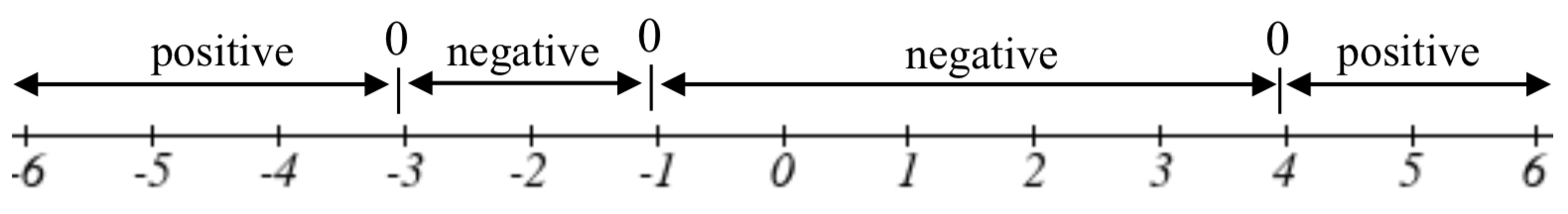
From our test values, we can determine this function is positive when \(x < -3\) or \(x > 4\), or in interval notation, \((-\infty ,-3)\bigcup (4,\infty )\)

You Try \(\PageIndex{5}\)

Given the function \(g(x)=x^{3} -x^{2} -6x\) use the methods that we have learned so far to find the vertical & horizontal intercepts, determine where the function is negative and positive, describe the end behavior, and sketch the graph without technology.

Answer

Vertical intercept (0, 0), Horizontal intercepts (-2, 0), (0, 0), (3, 0)

The function is negative on (\(-\infty\), -2) and (0, 3)

The function is positive on (-2, 0) and (3,\(\infty\))

The leading term is \(x^{3}\) so as \(x\to -\infty\), \(g(x)\to -\infty\) and as\(x\to \infty\), \(g(x)\to \infty\)

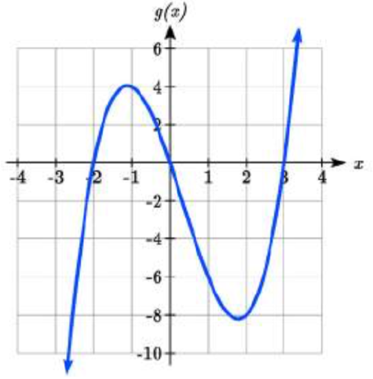
Figure \(\PageIndex{18}\): Graph of g(x)=x^3-x^2-6x