4.5: Zeros of Polynomials

Learning Objectives

• Find intervals that contain all real zeros.
• Use the Rational Zero Theorem to find rational zeros.
• Find zeros of a polynomial function.
• Write polynomial functions as a product of linear factors.
• Use Descartes’ Rule of Signs.
• Find polynomial functions that model given criteria.

In the previous section, we looked at the function \(f(x) = x^3 + 4x^2-5x-14\). We discussed how this function does not factor nicely using factoring techniques from intermediate algebra courses. We found from using technology that there was a "nice" x-intercept at \((2,0)\), "nice" meaning that the x-coordinate of the intercept was an integer value. We knew that this x-intercept came from a factor of \((x-2)\). We were then able to divide \(f\) by this factor to get the factored form of \(f\), \(f(x) = x^3 + 4x^2-5x-14=(x-2)(x^2+6x+7)\). Since the factor \(x^2+6x+7\) was quadratic, we are able to solve \(x^2+6x+7=0\) to find the other x-intercepts. If we did not have access to graphing technology or were unable to identify a "nice" x-intercept from graphing technology, how would be begin the process of finding zeros and factors of polynomials that do not factor nicely using techniques from intermediate algebra? This poses a real-life dilemma as we use polynomials when modeling many real-life situations.

In this section we will discuss some very important theory and techniques that will help us tackle this important question of finding zeros, also called roots, when polynomial functions do not factor "nicely." Let's begin with some useful theory that will help in determining intervals where we expect real zeros to be at as well as where me might start looking for possible "nice" zeros?

Bounds for Real Zeros

The theory below, which is due to the famous mathematician Augustin Cauchy, gives us an interval on which all of the real zeros of a polynomial can be found. This theory is useful since it guarantees us an interval where we can expect all our real zeros to be. Remember that real zeros correspond to x-intercepts on a graph.

Cauchy's Bound Theorem

Suppose

\[f(x) = a_{n} x^{n} + a_{n-1 }x^{n-1 } + \ldots + a_{1 } x + a_{0 } \nonumber \]

is a polynomial of degree \(n\) with \(n \geq 1\). Let \(M\) be the largest of the numbers:

\[\dfrac{|a_{0}|}{|a_{n}|}, \dfrac{|a_{1}|}{|a_{n}|}, \ldots, \dfrac{|a_{n-1}|}{|a_{n}|}\nonumber \]

Then all the real zeros of \(f\) lie in in the interval \([-(M+1),M+1]\).

The proof of this theorem is not easily explained within the confines of this text. Like many of the things discussed in this section, Cauchy's Bound Theorem is best understood with an example.

Example \(\PageIndex{1}\)

Let \(f(x) = 2x^4+4x^3-x^2-6x-3\). Determine an interval which contains all of the real zeros of \(f\).

Solution

To find the \(M\) stated in Cauchy's Bound, we take the absolute value of leading coefficient, in this case \(|2| = 2\) and divide it into the largest (in absolute value) of the remaining coefficients, in this case \(|-6| = 6\). We find \(M=3\), so it is guaranteed that the real zeros of \(f\) all lie in \([-4,4]\).

Cauchy's Bound is useful but it can provide us a very large interval when a polynomial has large coefficients in absolute value. The next theorem can be useful in finding a smaller interval where real zeros are within.

Upper and Lower Bounds Theorem

Suppose \(f\) is a polynomial of degree \(n \geq 1\).

• If \(c > 0\) is synthetically divided into \(f\) and all of the coefficients of the quotient and remainder are all non-negative values, then \(c\) is an upper bound for the real zeros of \(f\). That is, there are no real zeros greater than \(c\).
• If \(c < 0\) is synthetically divided into \(f\) and the coefficients of the quotient and remainder alternate signs, then \(c\) is a lower bound for the real zeros of \(f\). That is, there are no real zeros less than \(c\).

If the number \(0\) occurs as a coefficient of the quotient or remainder in the final line of the division table in either of the above cases, it can be treated as \((+)\) or \((-)\) as needed.

You may be wondering how to determine what value to use for \(c\) in the previous theorem. There is no systematic method for finding a \(c\) value to try, just pick a number and divide to see if it is an upper or lower bound for the real zeros.

Example \(\PageIndex{2}\)

Given \(P(x)=2x^4+27x^3-68x^2-333x+180\), use the Upper and Lower Bounds Theorem to find an interval which contains all of the real zeros of \(P\) that is smaller than the interval found using Cauchy's Bound Theorem.

Solution

From Cauchy's Bound, \(|a_{n}|=|2| = 2\). The largest coefficient in absolute value is \(|-333| = 333\). Then \(M=\dfrac{333}{2}=166.5\). All the real zeros lie in \([-167.5,167.5]\). We can see that this is a pretty large interval. This is where finding upper and lower bounds using the Upper and Lower Bounds Theorem can be helpful as it could give us a much smaller interval.

Let's begin with finding an upper bound. Let's try \(c=10\).

\( \begin{array}{l|lllll}
10 & 2 & 27 & -68 & -333 & 180 \\
& & 20 & 470 & 4020 & 36870 \\
\hline & 2 & 47 & 402 & 3687 & 37050
\end{array} \)

We can see that 10 is an upper bound for the real zeros of \(P\) since all the numbers on the last row of the table are all non-negative (which are the coefficients of the quotient and remainder). This is a significant improvement from Cauchy's Bound. Note that if 10 was not an upper bound, then we would pick another c value larger than 10 to test. We'd continue this process until we find a value that is an upper bound.

Next, let's find a lower bound. Let's pick \(c=- 10\).

\(\begin{array}{r|rrrrr}
-10 & 2 & 27 & -68 & -333 & -180 \\
& & -20 & -70 & 1380 & -1047 \\
\hline & 2 & 7 & -138 & 1047 & -10290
\end{array}\)

-10 is not a lower bound since the numbers on the last row of the table do not alternate signs between + and -. This indicates we must pick a number smaller to test. Let's try \(c=- 20\).

\(\begin{array}{r|rrrrr}
-20 & 2 & 27 & -68 & -333 & -180 \\
& & -40 & 260 & -3840 & 83460 \\
\hline & 2 & -13 & 192 & -4173 & 83640
\end{array}\)

Since the numbers on the last row of the table alternate signs between + and -, we can conclude that the real zeros will be in \([-20,10]\).

Do note that this interval is not unique as there are other values of c that will work.

Next, let's look at some theory that will help in providing a list of values that could be potential zeros for a polynomial.

Rational Zeros

Recall that rational numbers are numbers that can be written in the form \(\dfrac{a}{b}\) where \(a\) and \(b\) are integers.

The Rational Zeros Theorem

If a polynomial \(f(x)=a_nx^n+a_{n−1}x^{n−1}+...+a_1x+a_0\) has integer coefficients, then every rational zero of \(f(x)\) has the form \(\frac{p}{q}\) where \(p\) is a factor of the constant term \(a_0\) and \(q\) is a factor of the leading coefficient \(a_n\).

Example \(\PageIndex{3}\)

List all possible rational zeros of \(f(x)=2x^4−5x^3+x^2−4\).

Solution

The only possible rational zeros of \(f(x)\) are the quotients of the factors of the last term, –4, and the factors of the leading coefficient, 2.

The constant term is –4; the factors of –4 are \(p=±1,±2,±4\).

The leading coefficient is 2; the factors of 2 are \(q=±1,±2\).

If any of the four real zeros are rational zeros, then they will be of one of the following factors of –4 divided by one of the factors of 2.

\[\dfrac{p}{q}=±\dfrac{1}{1},±\dfrac{1}{2} \; \; \; \; \; \; \frac{p}{q}=±\dfrac{2}{1},±\dfrac{2}{2} \; \; \; \; \; \; \dfrac{p}{q}=±\dfrac{4}{1},±\dfrac{4}{2} \nonumber \]

Note that \(\frac{2}{2}=1\) and \(\frac{4}{2}=2\), which have already been listed. So we can shorten our list.

\[\dfrac{p}{q} = \dfrac{\text{Factors of the constant term}}{\text{Factors of the leading coefficient}}=±1,±2,±4,±\dfrac{1}{2}\nonumber \]

Example \(\PageIndex{4}\)

Use the Rational Zero Theorem to find the rational zeros of \(f(x)=2x^3+x^2−4x+1\).

Solution

The factors of the constant term are ±1 and the factors of the leading coefficient are ±1 and ±2. The possible values for \(\frac{p}{q}\) are ±1 and \(±\frac{1}{2}\). These are all the possible rational zeros for the function. We can determine which of these are actual zeros by substituting these values for \(x\) in \(f(x)\).

\[f(−1)=2{(−1)}^3+{(−1)}^2−4(−1)+1=4\nonumber \]

\[f(1)=1{(1)}^3+{(1)}^2−4(1)+1=0\nonumber \]

\[f\left(−\dfrac{1}{2}\right)=2{\left(−\dfrac{1}{2}\right)}^3+{\left(−\dfrac{1}{2}\right)}^2−4\left(−\dfrac{1}{2}\right)+1=3\nonumber \]

\[f\left(\dfrac{1}{2}\right)=2{\left(\dfrac{1}{2}\right)}^3+{\left(\dfrac{1}{2}\right)}^2−4\left(\dfrac{1}{2}\right)+1=−\dfrac{1}{2}\nonumber \]

1 is the only rational zero of \(f(x)\).

Example \(\PageIndex{5}\)

Find the rational zeros of \(f(x)=4x^3−3x−1\).

Solution

The factors of the constant term are ±1 and the factors of the leading coefficient are ±1, ±2, and ±4. The possible values for \(\dfrac{p}{q}\) are \(±1\),\(±\dfrac{1}{2}\), and \(±\dfrac{1}{4}\). These are the possible rational zeros for the function. Let’s begin with 1. \(f(1)=4(1)^3-3(1)-1=0\) so 1 is a zero of \(f\). Dividing by \((x−1)\) gives us the following factor for the polynomial:

\[(x−1)(4x^2+4x+1) \nonumber \]

The quadratic is a perfect square. \(f(x)\) can be written as

\[(x−1){(2x+1)}^2 \nonumber \]

We already know that 1 is a zero. The other zero will have a multiplicity of 2 because the factor is squared. To find the other zero, we can set the factor equal to 0.

\[ \begin{align*} 2x+1 &=0 \\[4pt] x &=−\dfrac{1}{2} \end{align*}\]

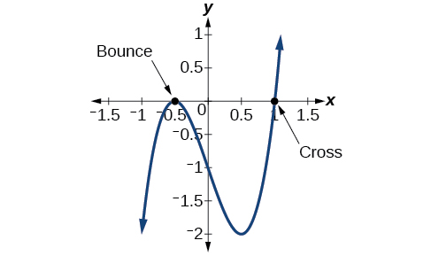
The zeros of the function are 1 and \(−\frac{1}{2}\) with multiplicity 2.

Analysis

Look at the graph of the function \(f\) in Figure \(\PageIndex{1}\). Notice, at \(x =−0.5\), the graph bounces off the x-axis, indicating the even multiplicity (2,4,6…) for the zero −0.5. At \(x=1\), the graph crosses the x-axis, indicating the odd multiplicity (1,3,5…) for the zero \(x=1\).

Figure \(\PageIndex{1}\): Graph of \(f(x)=4x^3−3x−1\)

You Try \(\PageIndex{1}\)

Use the Rational Zero Theorem to find the rational zeros of \(f(x)=x^3−5x^2+2x+1\).

Answer

There are no rational zeros for this function.

The Fundamental Theorem of Algebra

The Fundamental Theorem of Algebra tells us that every polynomial function has at least one complex zero. This theorem forms the foundation for solving polynomial equations.

Suppose \(f\) is a polynomial function of degree four, and \(f (x)=0\). The Fundamental Theorem of Algebra states that there is at least one complex solution, call it \(c_1\). By the Factor Theorem, we can write \(f(x)\) as a product of \(x−c_1\) and a polynomial quotient. Since \(x−c_1\) is linear, the polynomial quotient will be of degree three. Now we apply the Fundamental Theorem of Algebra to the third-degree polynomial quotient. It will have at least one complex zero, call it \(c_2\). So we can write the polynomial quotient as a product of \(x−c_2\) and a new polynomial quotient of degree two. Continue to apply the Fundamental Theorem of Algebra until all of the zeros are found. There will be four of them and each one will yield a factor of \(f(x)\).

The Fundamental Theorem Of Algebra

If \(f(x)\) is a polynomial of degree \(n > 0\), then \(f(x)\) has at least one complex zero.

Example \(\PageIndex{6}\)

Find the zeros of \(f(x)=3x^3+9x^2+x+3\).

Solution

The Rational Zero Theorem tells us that if \(\frac{p}{q}\) is a zero of \(f(x)\), then \(p\) is a factor of 3 and \(q\) is a factor of 3.

\[ \begin{align*} \dfrac{p}{q}&=\dfrac{\text{factors of constant term}}{\text{factors of leading coefficient}} \\[4pt] &=\dfrac{\text{factors of 3}}{\text{factors of 3}} \end{align*}\]

The factors of 3 are ±1 and ±3. The possible values for \(\dfrac{p}{q}\), and therefore the possible rational zeros for the function, are ±3,±1, and \(±\dfrac{1}{3}\). We will use synthetic division to evaluate each possible zero until we find one that gives a remainder of 0. Let’s begin with –3.

Dividing by \((x+3)\) gives a remainder of 0, so –3 is a zero of the function. The polynomial can be written as

\[(x+3)(3x^2+1) \nonumber\]

We can then set the quadratic equal to 0 and solve to find the other zeros of the function.

\[ \begin{align*} 3x^2+1&=0 \\[4pt] x^2 &=−\dfrac{1}{3} \\[4pt] x&=±−\sqrt{\dfrac{1}{3}} \\[4pt] &=±\dfrac{i\sqrt{3}}{3} \end{align*}\]

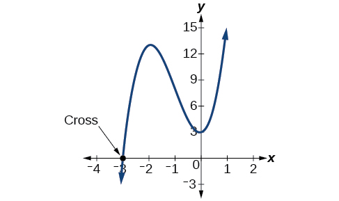
The zeros of \(f(x)\) are \(–3\) and \(±\dfrac{i\sqrt{3}}{3}\).

Analysis

Look at the graph of the function \(f\) in Figure \(\PageIndex{2}\). Notice that, at \(x =−3\), the graph crosses the x-axis, indicating an odd multiplicity (1) for the zero \(x=–3\). Also note the presence of the two turning points. This means that, since there is a \(3^{rd}\) degree polynomial, we are looking at the maximum number of turning points. So, the end behavior of increasing without bound to the right and decreasing without bound to the left will continue. Thus, all the x-intercepts for the function are shown. So either the multiplicity of \(x=−3\) is 1 and there are two complex solutions, which is what we found, or the multiplicity at \(x =−3\) is three. Either way, our result is correct.

Figure \(\PageIndex{2}\): Graph of \(f(x)=3x^3+9x^2+x+3\)

A vital implication of the Fundamental Theorem of Algebra, as we stated above, is that a polynomial function of degree n will have \(n\) zeros in the set of complex numbers, if we allow for multiplicities. This means that we can factor the polynomial function into \(n\) factors. As a result of this, the Linear Factorization Theorem tells us that a polynomial function will have the same number of factors as its degree, and that each factor will be in the form \((x−c)\), where c is a complex number.

Let \(f\) be a polynomial function with real coefficients, and suppose \(a +bi\), \(b≠0\), is a zero of \(f(x)\). Then, by the Factor Theorem, \(x−(a+bi)\) is a factor of \(f(x)\). For \(f\) to have real coefficients, \(x−(a−bi)\) must also be a factor of \(f(x)\). This is true because any factor other than \(x−(a−bi)\), when multiplied by \(x−(a+bi)\), will leave imaginary components in the product. Only multiplication with conjugate pairs will eliminate the imaginary parts and result in real coefficients. In other words, if a polynomial function \(f\) with real coefficients has a complex zero \(a +bi\), then the complex conjugate \(a−bi\) must also be a zero of \(f(x)\). This is called the Complex Conjugate Theorem.

Linear Factorization Theorem

If \(f(x)\) is a polynomial of degree \(n >0\), and a is a non-zero real number, then \(f(x)\) has exactly \(n\) linear factors

\[f(x)=a(x−c_1)(x−c_2)...(x−c_n) \nonumber \]

where \(c_1,c_2\),...,\(c_n\) are complex numbers.

\(f(x)\) has \(n\) zeros total when we allow for multiplicities.

Complex Conjugate Theorem

If the polynomial function \(f\) has real coefficients and a complex zero in the form \(a+bi\), then the complex conjugate of the zero, \(a−bi\), is also a zero.

Q&A

If \(2+3i\) were given as a zero of a polynomial with real coefficients, would \(2−3i\) also need to be a zero?

Yes. When any complex number with an imaginary component is given as a zero of a polynomial with real coefficients, the conjugate must also be a zero of the polynomial.

Example \(\PageIndex{7}\)

Find a fourth degree polynomial with real coefficients that has zeros of \(–3\), \(2\), \(i\), such that \(f(−2)=100\).

Solution

Because \(x =i\) is a zero, by the Complex Conjugate Theorem \(x =–i\) is also a zero. The polynomial must have factors of \((x+3),(x−2),(x−i)\), and \((x+i)\). Since we are looking for a degree 4 polynomial, and now have four zeros, we have all four factors. Let’s begin by multiplying these factors.

\[\begin{align*} f(x) & =a(x+3)(x−2)(x−i)(x+i) \\ f(x) & =a(x^2+x−6)(x^2+1) \\ f(x) & =a(x^4+x^3−5x^2+x−6) \end{align*} \nonumber \]

We need to find \(a\) to ensure \(f(–2)=100\). Substitute \(x=–2\) and \(f (-2)=100\) into \(f (x)\).

\[\begin{align*} 100=a({(−2)}^4+{(−2)}^3−5{(−2)}^2+(−2)−6) \\ 100=a(−20) \\ −5=a \end{align*} \nonumber \]

So the polynomial function is

\[f(x)=−5(x^4+x^3−5x^2+x−6)\nonumber \]

or

\[f(x)=−5x^4−5x^3+25x^2−5x+30\nonumber \] Analysis

We found that both \(i\) and \(−i\) were zeros, but only one of these zeros needed to be given. If \(i\) is a zero of a polynomial with real coefficients, then \(−i\) must also be a zero of the polynomial because \(−i\) is the complex conjugate of \(i\).

Example \(\PageIndex{8}\)

Let \(f(x) = 12x^5 - 20x^4+19x^3-6x^2-2x+1\).

1. Find all of the complex zeros of \(f\) and state their multiplicities.
2. Write \(f(x)\) as a product of linear factors.

Solution

1.Since \(f\) is a fifth degree polynomial, we know that we need to perform at least three successful divisions to get the quotient down to a quadratic function. At that point, we can find the remaining zeros using the Quadratic Formula, if necessary. Using the techniques developed in Section 3.3, we get

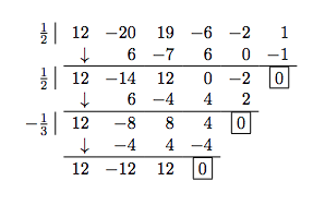
Our quotient is \(12x^2 - 12x + 12\), whose zeros we find to be \(\frac{1 \pm i \sqrt{3}}{2}\). From Theorem 3.14, we know \(f\) has exactly \(5\) zeros, counting multiplicities, and as such we have the zero \(\frac{1}{2}\) with multiplicity \(2\), and the zeros \(-\frac{1}{3}\), \(\frac{1 + i \sqrt{3}}{2}\) and \(\frac{1 - i \sqrt{3}}{2}\), each of multiplicity \(1\).

2. Applying th eLinear Factorization Theorem, we are guaranteed that \(f\) factors as

\[f(x) = 12 \left(x- \dfrac{1}{2}\right)^2 \left(x + \dfrac{1}{3}\right) \left(x - \left[\dfrac{1 + i \sqrt{3}}{2}\right]\right) \left(x - \left[\dfrac{1 - i \sqrt{3}}{2}\right]\right)\nonumber \]

A true test of the Linear Factorization Theorem (and a student's mettle!) would be to take the factored form of \(f(x)\) in the previous example and multiply it out {You really should do this once in your life to convince yourself that all of the theory actually does work!} to see that it really is the original function

\[f(x) = 12x^5 - 20x^4+19x^3-6x^2-2x+1.\nonumber \]

When factoring a polynomial using the Linear Factorization Theorem, we say that it is factored completely over the complex numbers, meaning that it is impossible to factor the polynomial any further using complex numbers. If we wanted to completely factor \(f(x)\) over the real numbers then we would have stopped short of finding the nonreal zeros of \(f\) and factored \(f\) using our work from the synthetic division to write

\[f(x) = \left(x - \frac{1}{2} \right)^2 \left(x + \frac{1}{3} \right)\left(12x^2 - 12x + 12\right)\nonumber \]

or

\[(f(x) = 12\left(x - \frac{1}{2} \right)^2 \left(x + \frac{1}{3} \right)\left(x^2 - x + 1\right).\nonumber \]

Since the zeros of \(x^2-x+1\) are nonreal, we call \(x^2-x+1\) an irreducible quadratic meaning it is impossible to break it down any further using real numbers.

The last two results of the section show us that, at least in theory, if we have a polynomial function with real coefficients, we can always factor it down enough so that any nonreal zeros come from irreducible quadratics.

Descartes' Rule of Signs

The process of testing possible rational zeros and dividing can be tedious for some polynomial functions. There is a straightforward way to determine the possible numbers of positive and negative real zeros for any polynomial function. If the polynomial is written in descending order, Descartes’ Rule of Signs tells us of a relationship between the number of sign changes in \(f(x)\) and the number of positive real zeros. For example, the polynomial function below has one sign change.

This tells us that the function must have 1 positive real zero.

There is a similar relationship between the number of sign changes in \(f(−x)\) and the number of negative real zeros.

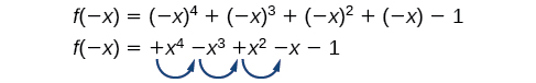
In this case, \(f(−x)\) has 3 sign changes. This tells us that \(f(x)\) could have 3 or 1 negative real zeros.

Theorem: Descartes' Rule of Signs

Suppose \(f(x)\) is the formula for a polynomial function written with descending powers of \(x\).

1. If \(P\) denotes the number of variations of sign in the formula for \(f(x)\), then the number of positive real zeros (counting multiplicity) is one of the numbers \(P, P-2, P-4, \ldots \).
2. If \(N\) denotes the number of variations of sign in the formula for \(f(-x)\), then the number of negative real zeros (counting multiplicity) is one of the numbers \{N\), \(N-2\), \(N-4\), \dots\}.
3. All other zeros are complex zeros.

Example \(\PageIndex{9}\)

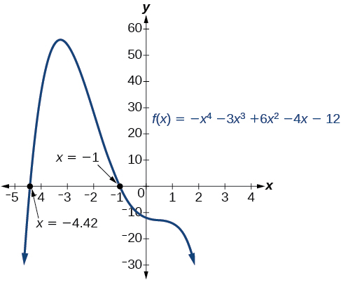
Use Descartes’ Rule of Signs to determine the possible numbers of positive and negative real zeros for \(f(x)=−x^4−3x^3+6x^2−4x−12\).

Solution

Begin by determining the number of sign changes.

There are two sign changes for \(f(x)\), so there are either 2 or 0 positive real roots.

Next, we examine \(f(−x)\) to determine the number of negative real roots.

\[ \begin{align*} f(−x) & =−{(−x)}^4−3{(−x)}^3+6{(−x)}^2−4(−x)−12 \\ f(−x) & =−x^4+3x^3+6x^2+4x−12 \end{align*} \nonumber\]

Again, there are two sign changes for \(f(-x)\), so there are either 2 or 0 negative real roots.

There are four possibilities, as we can see in Table \(\PageIndex{1}\).

Table \(\PageIndex{1}\)

Positive Real Zeros	Negative Real Zeros	Complex Zeros	Total Zeros
2	2	0	4
2	0	2	4
0	2	2	4
0	0	4	4

Analysis

We can confirm the numbers of positive and negative real roots by examining a graph of the function. See Figure \(\PageIndex{3}\). We can see from the graph that the function has 0 positive real roots and 2 negative real roots.

Figure \(\PageIndex{3}\): Graph of \(f(x)=−x^4−3x^3+6x^2−4x−12\) with x-intercepts at \((-4.42,0)\) and \((-1,0)\)

You Try \(\PageIndex{2}\)

Use Descartes’ Rule of Signs to determine the maximum possible numbers of positive and negative real zeros for \(f(x)=2x^4−10x^3+11x^2−15x+12\).

Solution

There must be 4, 2, or 0 positive real roots and 0 negative real roots. The graph shows that there are 2 positive real zeros and 0 negative real zeros.

Example \(\PageIndex{10}\)

Let \(f(x) = 2x^4+4x^3-x^2-6x-3\).

1. Find all of the zeros of \(f\) and their multiplicities.
2. Sketch the graph of \(y=f(x)\).

Solution

1. We know from Cauchy's Bound that all of the real zeros lie in the interval \([-4,4]\) and that our possible rational zeros are \(\pm \, \frac{1}{2}\), \(\pm \, 1\), \(\pm \, \frac{3}{2}\) and \(\pm \, 3\). Descartes' Rule of Signs guarantees us at least one negative real zero and exactly one positive real zero, counting multiplicity. We try our positive rational zeros, starting with the smallest, \(\frac{1}{2}\). Since the remainder isn't zero, we know \(\frac{1}{2}\) isn't a zero. Sadly, the final line in the division tableau has both positive and negative numbers, so \(\frac{1}{2}\) is not an upper bound. The only information we get from this division is courtesy of the Remainder Theorem which tells us \(f\left(\frac{1}{2}\right) = -\frac{45}{8}\) so the point \(\left(\frac{1}{2}, -\frac{45}{8}\right)\) is on the graph of \(f\). We continue to our next possible zero, \(1\). As before, the only information we can glean from this is that \((1,-4)\) is on the graph of \(f\). When we try our next possible zero, \(\frac{3}{2}\), we get that it is not a zero, and we also see that it is an upper bound on the zeros of \(f\), since all of the numbers in the final line of the division tableau are positive. This means there is no point trying our last possible rational zero, \(3\). Descartes' Rule of Signs guaranteed us a positive real zero, and at this point we have shown this zero is irrational. Furthermore, the Intermediate Value Theorem, Theorem 3.1, tells us the zero lies between \(1\) and \(\frac{3}{2}\), since \(f(1) < 0\) and \(f\left(\frac{3}{2}\right) > 0\).

\(\begin{array}{rrrrrr} \frac{1}{2} \mid & 2 & 4 & -1 & -6 & -3 \\ & \quad  \downarrow & 1 & \frac{5}{2} & \frac{3}{4} & -\frac{21}{8} \\\hline & 2 & 5 & \frac{3}{2} & -\frac{21}{4} & -\frac{45}{8} \end{array}\)

\( \begin{array}{rrrrr} 1 \mid  2 & 4 & -1 & -6 & -3 \\ \downarrow & 2 & 6 & 5 & -1 \\ \hline 2 & 6 & 5 & -1 & -4 \end{array}\)

\(\begin{array}{r|rrrrr} \frac{3}{2}  & 2 & 4 & -1 & -6 & -3 \\ &\downarrow & 3 & \frac{21}{2} & \frac{57}{4} & \frac{99}{8} \\ \hline &2 & 7 & \frac{19}{2} & \frac{33}{4} & \frac{75}{8} \end{array}\)

 

2. We now turn our attention to negative real zeros. We try the largest possible zero, \(-\frac{1}{2}\). Synthetic division shows us it is not a zero, nor is it a lower bound (since the numbers in the final line of the division tableau do not alternate), so we proceed to \(-1\). This division shows \(-1\) is a zero. Descartes' Rule of Signs told us that we may have up to three negative real zeros, counting multiplicity, so we try \(-1\) again, and it works once more. At this point, we have taken \(f\), a fourth degree polynomial, and performed two successful divisions. Our quotient polynomial is quadratic, so we look at it to find the remaining zeros.

\(\begin{array}{r|rrrrr} -\frac{1}{2} & 2 & 4 & -1 & -6 & -3 \\ &\downarrow & -1 & -\frac{3}{2} & \frac{5}{4} & \frac{19}{8} \\ \hline &2 & 3 & -\frac{5}{2} & -\frac{19}{4} & -\frac{5}{8} \end{array}\)

\(\begin{array}{rrrrrr} -1 \mid & 2 & 4 & -1 & -6 & -3 \\ & \downarrow & -2 & -2 & 3 & 3 \\ \hline \end{array}\) \( \begin{array}{rrrrr} -1 \mid & 2 & 2 & -3 & -3 \\ &\downarrow & -2 & 0 & 3 \\ \hline & 2 & 0 & -3 & 0 \end{array} \)

Setting the quotient polynomial equal to zero yields \(2x^2 - 3 = 0\), so that \(x^2 = \frac{3}{2}\), or \(x = \pm \, \frac{\sqrt{6}}{2}\). Descartes' Rule of Signs tells us that the positive real zero we found, \(\frac{\sqrt{6}}{2}\), has multiplicity \(1\). Descartes also tells us the total multiplicity of negative real zeros is \(3\), which forces \(-1\) to be a zero of multiplicity \(2\) and \(- \frac{\sqrt{6}}{2}\) to have multiplicity \(1\).

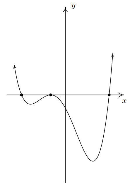
We know the end behavior of \(y=f(x)\) resembles that of its leading term \(y=2x^4\). This means that the graph enters the scene in Quadrant II and exits in Quadrant I. Since \(\pm \, \frac{\sqrt{6}}{2}\) are zeros of odd multiplicity, we have that the graph crosses through the \(x\)-axis at the points \(\left( -\frac{\sqrt{6}}{2}, 0 \right)\) and \(\left( \frac{\sqrt{6}}{2}, 0 \right)\). Since \(-1\) is a zero of multiplicity \(2\), the graph of \(y=f(x)\) touches and rebounds off the \(x\)-axis at \((-1,0)\). Putting this together, we get the graph of \(f\) below in Figure \(\PageIndex{4}\)

Figure \(\PageIndex{4}\): Graph of \(f(x)=2x^4+4x^3-x^2-6x-3\)

Our last example turns the tables and asks us to manufacture a polynomial with certain properties of its graph and zeros.

Example \(\PageIndex{11}\)

Find a polynomial \(p\) of lowest degree that has integer coefficients and satisfies all of the following criteria:

1. the graph of \(y=p(x)\) touches (but does not cross) the \(x\)-axis at \(\left(\frac{1}{3}, 0\right)\)
2. \(x=3i\) is a zero of \(p\).
3. as \(x \rightarrow -\infty\), \(p(x) \rightarrow -\infty\)
4. as \(x \rightarrow \infty\), \(p(x) \rightarrow -\infty\)

Solution

To solve this problem, we will need a good understanding of the relationship between the \(x\)-intercepts of the graph of a function and the zeros of a function, the Factor Theorem, the role of multiplicity, complex conjugates, the Complex Factorization Theorem, and end behavior of polynomial functions. (In short, you'll need most of the major concepts of this chapter.) Since the graph of \(p\) touches the \(x\)-axis at \(\left(\frac{1}{3}, 0\right)\), we know \(x=\frac{1}{3}\) is a zero of even multiplicity. Since we are after a polynomial of lowest degree, we need \(x=\frac{1}{3}\) to have multiplicity exactly \(2\).

The Factor Theorem now tells us \(\left(x-\frac{1}{3}\right)^2\) is a factor of \(p(x)\). Since \(x=3i\) is a zero and our final answer is to have integer (real) coefficients, \(x=-3i\) is also a zero. The Factor Theorem kicks in again to give us \((x-3i)\) and \((x+3i)\) as factors of \(p(x)\). We are given no further information about zeros or intercepts so we conclude, by the Complex Factorization Theorem that \(p(x) = a \left(x-\frac{1}{3}\right)^2 (x-3i)(x+3i)\) for some real number \(a\). Expanding this, we get

\[p(x) = ax^4-\frac{2a}{3} x^3+\frac{82a}{9} x^2-6ax+a \nonumber\]

In order to obtain integer coefficients, we know \(a\) must be an integer multiple of \(9\). Our last concern is end behavior. Since the leading term of \(p(x)\) is \(ax^4\), we need \(a < 0\) to get \(p(x) \rightarrow -\infty\) as \(x \rightarrow \pm \infty\). Hence, if we choose \(x=-9\), we get

\[p(x) = -9x^4+ 6 x^3 - 82 x^2+54x-9 \nonumber\]

We can verify our handiwork using the techniques developed in this chapter.

This example concludes our study of polynomial functions. The last few sections have contained what is considered by many to be 'heavy' Mathematics. Like a heavy meal, heavy Mathematics takes time to digest. Don't be overly concerned if it does not seem to sink in all at once and pace yourself as you practice. With time and dedication you've got this!