
4.7: Graphing Rational Functions
- Page ID
- 89428

- Identify important behavior of rational functions and use this information to sketch their graphs.
- Find equations of rational functions that model graphical information.
In this section we are going look at sketching graphs of rational functions. Although technology can graph functions for us, it is important that we understand the details of how these functions behave. Window settings for viewing a graph in a graphing calculator can significantly affect what graphical behavior we see. What if you owned a company that produced and sold cookies. Your company would have some costs to produce cookies. In business, it is known that average cost models are rational functions. As a business owner, you’d want to reduce your costs as much as possible. This means you’d want to find the smallest of the local minimums for the functions. If you didn’t know how the function model for your costs behaved, how would you be certain you had reduced your costs as much as possible? This is just one of many examples of why it is important to understand how functions behave.
Graphing Rational Functions
Let’s take a moment to review what we know about rational function behavior. Rational functions have vertical asymptotes or holes for values not in the domain of the function. We know the function values increase or decrease without bound as we near vertical asymptotes. Rational functions have horizontal, slant, or oblique asymptotes which are polynomials that we can use to describe their end behavior. On the ends of the graph, the function will approach one of these asymptotes. To figure out how the function behaves elsewhere, we can use points such as intercepts and also sign charts.
Let \(r(x)\) be a rational function.
- Write \(r\) as a single fraction in factored form.
- Determine the domain of \(r\).
- Find the vertical asymptotes of \(r\), if any.
- Find any holes in the graph, if they exist.
- Find the horizontal, slant, or oblique asymptote for \(r\).
- Find all intercepts for \(r\), if any.
- Find all points where the function intersects the horizontal or slant or oblique asymptote, if any.
- Use this information to sketch the graph of \(r(x)\). If needed, construct a sign chart and find other points to help with sketching the graph.
A note is in order about checking to see if \(r(x)\) intersects its horizontal or slant or oblique asymptote. Unlike vertical asymptotes that occur at values not in the domain of \(r(x)\), these asymptotes describe end behavior of the function only. This means that it is possible that \(r(x)\) can have the same function value as the horizontal or slant or oblique asymptote somewhere in between the ends. That is why we must check this.
For the given function, \(r(x)=\dfrac{x^2+2x-3}{x^2+2x-8}\),
- Find the domain and state answer in interval notation.
- Identify all the asymptotes, if any.
- Identify any holes in the graph of \(r\), if any.
- Describe the end behavior of \(r\) using proper notation.
- Find the x and y-intercepts.
- Set up a sign chart and use it to describe where \(r(x)>0\) and \(r(x)<0\).
- Use the information your found above to sketch a graph of \(r\).
- Find the range of \(r(x)\) and state answer in interval notation. Use graphing technology and round to the first decimal place, if applicable.
Solution
- To find domain, we first must factor: \[r(x)=\dfrac{x^2+2x-3}{x^2+2x-8}=\dfrac{(x+3)(x-1)}{(x-2)(x+4)}\nonumber\]From here we can see that \(x=2\) and \(x=-4\) will make \(r\) undefined. Hence, the domain is \((-\infty, -4) \cup (-4,2) \cup (2,\infty)\).
- Since there are no common factors between the numerator and denominator we can conclude that there are two vertical asymptotes at \(x=2\) and \(x=-4\). The degree of the numerator and denominator are the same, degree 2, so there is a horizontal asymptote at \(y=\dfrac{1}{1}=1\).
Remember that we do need to check if the function intersects the horizontal asymptote so let's check this. To do so, we need to find out if there are any points for \(r(x)\) that have a y-coordinate equal to 1. To find out, set \(r(x)=1\)\[\dfrac{x^2+2x-3}{x^2+2x-8}=1\nonumber \]Multiplying both sides by the common denominator, \[(x^2+2x-8)\left(\dfrac{x^2+2x-3}{x^2+2x-8}\right)=(x^2+2x-8)(1)\nonumber\]which simplifies to \[x^2+2x-3=x^2+2x-8\nonumber\]Subtracting \(x^2\) and then \(2x\) from both sides yields \[-3=-8\nonumber\]which is a false statement. We can conclude that \(r\) does not intersect it's horizontal asymptote.
- Since there are no common factors between the numerator and denominator, we can conclude there are no holes in the graph of \(r(x)\).
- As \(x \rightarrow \pm \infty\), \(r(x) \rightarrow 1\).
- To find the x-intercepts set \(y=0\), \[\dfrac{x^2+2x-3}{x^2+2x-8}=0\nonumber\]Multiplying both sides by the common denominator, \[(x^2+2x-8)(\dfrac{x^2+2x-3}{x^2+2x-8})=(x^2+2x-8)(0)\nonumber\]which simplifies to \[x^2+2x-3=0 \nonumber \]Notice that this is just the numerator or \(r(x)\). Now factoring, \[(x+3)(x-1)=0\nonumber\]which gives us \(x=-3\) and \(x=1\). The x-intercepts are \((-3,0)\) and \((1,0)\).
To find the y-intercept, evaluate the function at \(x=0\)\[r(0)=\dfrac{(0)^2+2(0)-3}{(0)^2+2(0)-8}=\dfrac{-3}{-8}=\dfrac{3}{8}\nonumber\]The y-intercept is \(\left(0, \dfrac{3}{8}\right)\).
Note that for the x-intercepts we can just look at the factored numerator of \(r(x)\) without having to actually go through the steps of solving \(r(x)=0\). Keep this in mind as this can save you some time! Also notice that for the y-intercept, the y-coordinate is just the constant terms of the numerator and denominator of \(r(x)\) in unfactored form.
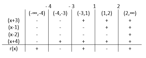
- The critical values for \(r(x)\) are -4, -3, 1, and 2. Setting up a sign chart:
.png?revision=1)
\(r(x)>0\) on the intervals \((-\infty, -4)\), \((-3, 1)\), and \((2,\infty)\)
\(r(x)<0\) on the intervals \((-4, -3)\) and \((1, 2)\)
- We begin by sketching dashed lines for the vertical asymptotes of \(r(x)\). We use dashed lines since asymptotes describe behavior of the function but they are not actually part of the graph of the function. We know that \(r(x)\) will increase or decrease without bound as the graph nears the vertical asymptotes so we can indicate this behavior on our graph, as shown in Figure \(\PageIndex{2}\).
_near_them.png?revision=1&size=bestfit&width=481&height=487)
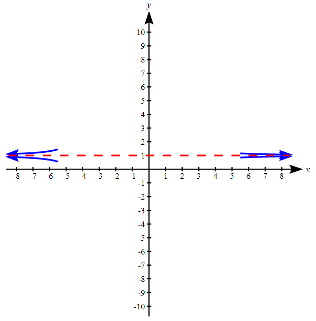
Next, we sketch a dashed line for the horizontal asymptote. We know that as \(x \rightarrow \pm \infty\), \(r(x) \rightarrow 1\), so we can indicate this behavior on our graph, as shown in Figure \(\PageIndex{3}\).
_and_end_behavior.png?revision=1&size=bestfit&width=489&height=497)
Now add the intercepts to the graph, as shown in Figure \(\PageIndex{4}\)
.png?revision=1&size=bestfit&width=479&height=497)
Since the domain is \((-\infty, -4) \cup (-4,2) \cup (2,\infty)\) there will be three parts to the graph, one part on each interval. On the interval \((-\infty, -4)\), we know that there are no x-intercepts and that the graph does not intersect the horizontal asymptote. This tells us that the graph must be above the horizontal asymptote. We can also see from the sign chart that \(r(x)>0\) on this interval which indicates the graph can not go below the x-axis. On the interval \((-4,2)\), we know the graph does not intersect the horizontal asymptote. This tells us that the graph must come from below the x-axis to be able to pass through the intercepts. On the interval \((2,\infty)\), we know that there are no x-intercepts and that the graph does not intersect the horizontal asymptote. This means that the graph must be above the horizontal asymptote here. We can also see from the sign chart that \(r(x)>0\) on this interval which indicates the graph can not go below the x-axis. The graph of \(r(x)\) is shown in Figure \(\PageIndex{5}\)
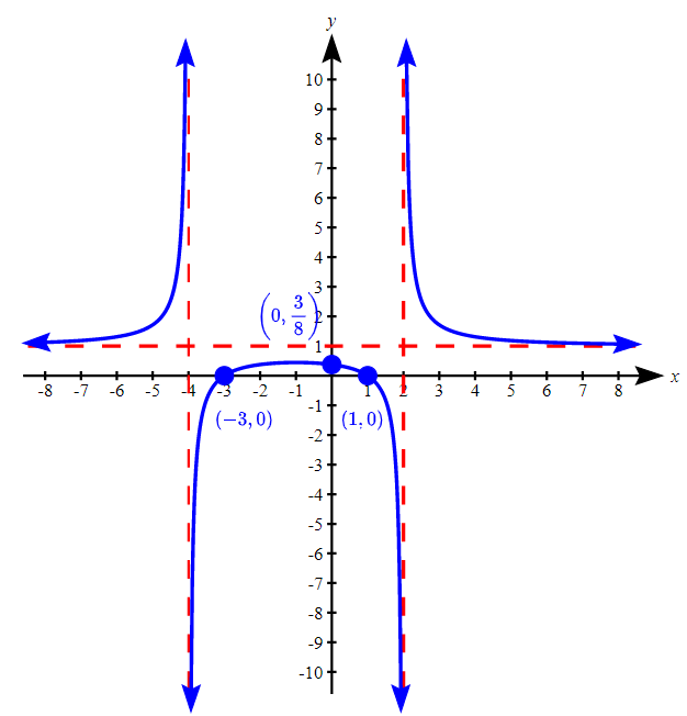.png?revision=2&size=bestfit&width=459&height=478)
- We can see that there is a local maximum within the interval \((-4,2)\) which we will need to approximate using a graphing calculator. The maximum occurs at approximately \((-1,0.4)\). Rounding to the nearest first decimal place, the range is \((-\infty,0.4] \cup (1,\infty)\).
In the previous example, we learned that we can find the x-intercepts quickly by looking at factors of the numerator. Do keep in mind that you must simplify the function first before determining the x-intercepts since there could be common factors between the numerator and denominator which would indicate that a hole exists.
Find the asymptotes, intercepts, domain, range, and end behavior of \(f(x)=\dfrac{3x^2+14x-5}{x+3}\). Round to the first decimal place for the range, if applicable. Then, use this information to sketch \(f(x)\).
Solution
Let's begin with factoring to determine the domain. \(f(x)=\dfrac{3x^2+14x-5}{x+3}=\dfrac{(x+5)(3x-1)}{x+3}\).
From the factored form of \(f(x)\), we find that the domain is \((-\infty,-3) \cup (-3,\infty)\). We can also tell from the factored that there is no hole and that there is a vertical asymptote at \(x=-3\).
Since there are no common factors between the numerator and denominator, we can set the numerator factors equal to 0 to find the x-intercepts, \((-5,0)\) and \((\dfrac{1}{3},0)\).
Evaluating at \(x=0\), \(f(0)=\dfrac{-5}{3}\) so the y-intercept is \(\left(-\dfrac{5}{3},0\right)\).
The degree of the numerator is one degree larger than the degree of the denominator so there is a slant asymptote. Using division, \[f(x)=\dfrac{3x^2+14x-5}{x+3}=3x+5-\dfrac{20}{x+3}\nonumber\]The slant asymptote is \(y=3x+5\).
Checking to see if \(f\) intersects its slant asymptote,
\[\begin{align*}\dfrac{3x^2+14x-5}{x+3} &=3x+5 \\[15pt] 3x^2+14x-5 &= (x+3)(3x+5) \qquad \text {multiply both sides by LCD} \\[15pt] 3x^2+14x-5 &= 3x^2+14x-15 \qquad \text {multiply}\\[15pt] -5 &=-15 \qquad \end{align*}\nonumber\]
This is a false statement so we can conclude that \(f\) does not intersect its slant asymptote.
Since the slant asymptote is a line with a positive slope, the end behavior is: as \(x \rightarrow -\infty\), \(f(x) \rightarrow -\infty\), and as \(x \rightarrow \infty\), \(f(x) \rightarrow \infty\).
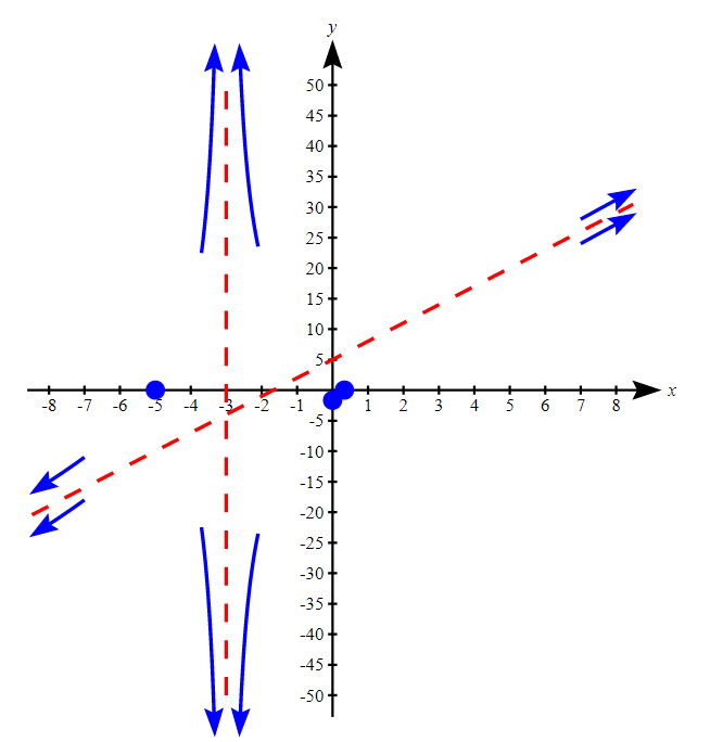
Next, sketch the the asymptotes as dashed lines. Fill in the behavior of \(f(x)\) near the asymptotes and plot the intercepts, as shown in Figure \(\PageIndex{6}\).
.png?revision=2&size=bestfit&width=457&height=478)
We know there is an x-intercept on the interval \((-\infty,-3)\) and that the graph does not intercept the slant asymptote. This tells us that the graph must be above the slant asymptote and that as \(x \rightarrow -3\), \(f(x) \rightarrow \infty\). We also know there there is an x and y-intercept on the interval \((-3,\infty)\) and that the graph does not intercept the slant asymptote on this interval. This tells us that the graph must be below the slant asymptote and that as \(x \rightarrow -3\), \(f(x) \rightarrow \infty\). The graph of \(f(x)\) is shown below in Figure \(\PageIndex{7}\).
.png?revision=1&size=bestfit&width=432&height=473)
Vertical asymptote at \(x=-3\), slant asymptote at \(y=3x+5\), intercepts at \((-5,0), \text{ } \left(\dfrac{1}{3},0\right) \text {, and } \left(0,-\dfrac{5}{3}\right)\), domain is \((-\infty,\infty)\), range is \((-\infty,\infty)\), and end behavior is as \(x \rightarrow -\infty\), \(f(x) \rightarrow -\infty\), and as \(x \rightarrow \infty\), \(f(x) \rightarrow \infty\).
Note that a sign chart and other points were not needed to help us determine the general shape of the graph of \(f(x)\) in the previous example. This is not always the case when sketching graphs of rational functions.
Find the asymptotes, intercepts, domain, range, and end behavior of \(B(x)=\dfrac{3x^2-7x-6}{x^2+3x-4}\). Round to the first decimal place for the range, if applicable. Then, use this information to sketch \(B(x)\).
- Answer
-
Vertical asymptotes at \(x=-4 \text{ and } x=1\), horizontal asymptote at \(y=3\), graph intersects horizontal asymptote at \(\left(\dfrac{3}{8},3\right)\),
intercepts at \(\left(-\dfrac{2}{3},0\right) \text{, } (3,0) \text{ and } \left(0,\dfrac{3}{2}\right)\),
domain is \((-\infty,-4) \cup (-4,1) \cup (4,\infty)\), range is \((-\infty,\infty)\), as \(x \rightarrow \pm \infty\), \(B(x) \rightarrow 3\).
The graph of \(B(x)\) is shown in Figure \(\PageIndex{8}\).
.png?revision=1&size=bestfit&width=419&height=431)
Figure \(\PageIndex{8}\): Graph of B(x)
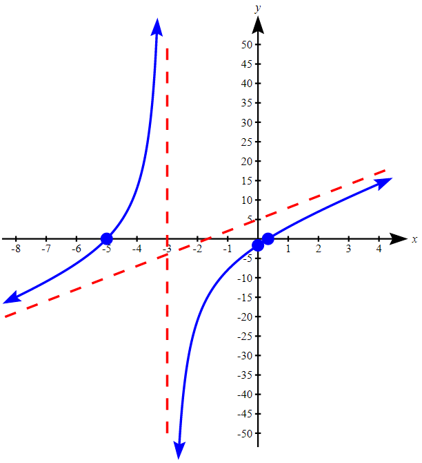
Find the asymptotes, intercepts, domain, range, and end behavior of \(g(t)=\dfrac{9t+9-t^3-t^2}{t^3+t^2+3t+3}\). Round to the first decimal place for the range, if applicable. Then, use this information to sketch \(g(t)\).
Solution
To begin, we need factor. Write terms in descending order and factoring by grouping,
\[g(t) =\dfrac{9t+9-t^3-t^2}{t^3+t^2+3t+3} = \dfrac{-(t+3)(t-3)(t+1)}{(t^2+3)(t+1)} \nonumber\]
Note that \(t^2+3\) does factor into \((t+\sqrt{3}i)(t-\sqrt{3}i)\) but we are graphing in a real coordinate system so we need not be concerned about these factors.
From the factored form of \(g(t)\), we find that the domain is \((-\infty,-1) \cup (-1,\infty)\). There is a hole at \((-1,2)\) (remember that the y-coordinate is found by simplifying the function first, then evaluating at -1 ). The t-intercepts are at \((-3,0) \text{ and } (3,0)\).
The y-intercept is \((0,3)\) since \(g(0)=\dfrac{9}{3}=3\).
There are no vertical asymptotes since there are no real numbers that make the denominator zero after simplifying.
There is a horizontal asymptote at \(y=-1\). Verify on your own that \(g\) does not intersect the horizontal asymptote.
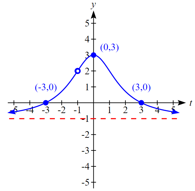
Sketch the the asymptote, points, and hole, as shown in Figure \(\PageIndex{9}\).
.png?revision=1&size=bestfit&width=379&height=381)
We are able to connect this information to sketch the curve, as shown in Figure \(\PageIndex{10}\), without further information since the points found are below the asymptote and we know that the graph does not intersect the asymptote.
.png?revision=1&size=bestfit&width=381&height=374)
No vertical asymptotes, horizontal asymptote at \(y=-1\), intercepts at \((-3,0) \text{, } (3,0) \text{, and } (0,3)\), hole at \((-1,2)\),
domain is \((-\infty,\infty)\), range is \((1,3]\), as \(x \rightarrow \pm \infty\), \(g(t) \rightarrow -1\).
Note that we know there is a local maximum from sketching the graph but we are unable to just assume that it is at the y-intercept. The graphing calculator helped us verify that there is a maximum at the y-intercept in this example. In calculus, you will learn ways to find local extrema without aid of graphing technology.
Find the asymptotes, intercepts, domain, and range of \(A(x)=\dfrac{x^2+6x-40}{2x^3-11x^2+10x+8} \). Round to the third decimal place for the range, if applicable. Then, use this information to sketch \(A(x)\).
Solution
First, factor \(A(x)\) (you will need to use some factoring techniques discussed recently to factor), \[A(x)=\dfrac{x^2+6x-40}{2x^3-11x^2+10x+8}=\dfrac{(x-4)(x+10)}{(x-4)(x-2)(2x+1)}\nonumber\]
From the factored form of \(A(x)\), we find the domain is \((-\infty,-\dfrac{1}{2}) \cup (-\dfrac{1}{2},2) \cup (2,4) \cup (4, \infty)\). There is a hole at \(\left(4,\dfrac{7}{9}\right)\).
There are vertical asymptotes at \(x=2 \text{ and } x=-\dfrac{1}{2}\).
There is a horizontal asymptote at \(y=0\). We do not need to check if \(A(x)\) intersects the asymptote as we gain this information when finding the x-intercepts since the horizontal asymptote is the x-axis.
The x-intercept is \((-10,0)\). The y-intercept is \((0,-5)\).
Sketch the the asymptote, points, and hole as shown in Figure \(\PageIndex{11}\).
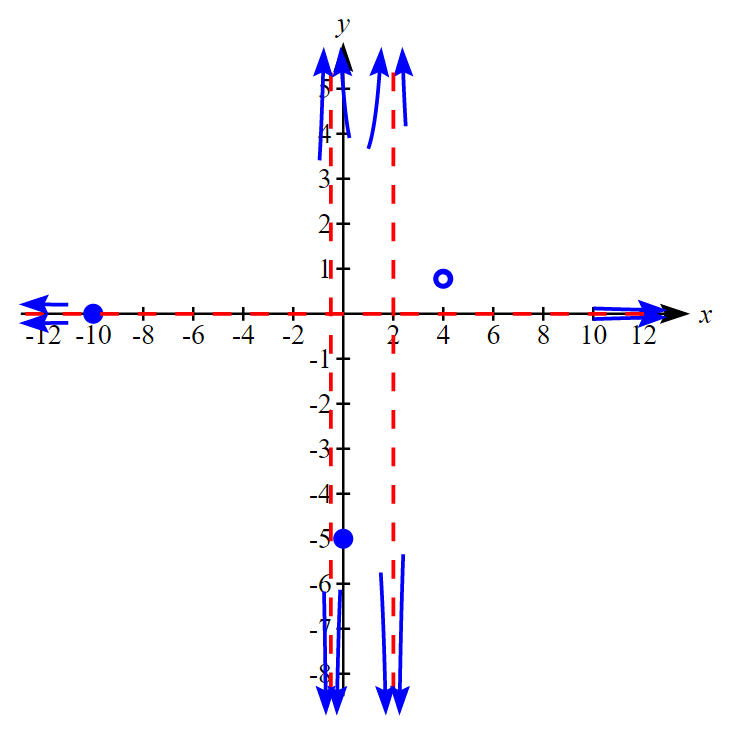.png?revision=1&size=bestfit&width=448&height=444)
On the interval \(\left(-\infty,-\dfrac{1}{2}\right)\), we know that as \(x \rightarrow -\infty \text{, } A \rightarrow 0\). Also, as \(x \rightarrow -\dfrac{1}{2}^-\), \(A \rightarrow -\infty\) or \(A \rightarrow \infty\). There is also an x-intercept at \((-10,0)\) within this interval. Applying what we have learned about polynomials, the graph must pass through the x-intercept since it comes from the factor \((x+10)\) which is a single root of multiplicity.
Currently, this is not enough information to sketch the graph on this interval since we do not know if the graph will be above or below the x-axis on the interval \((-\infty,-10)\). This is also the case for the interval \(\left(-10,-\dfrac{1}{2}\right)\). We can either set up a sign chart of find a point within one of these intervals to find out.
Using the latter, let's evaluate at \(x=-6\). \[A(-6)=\dfrac{1}{22}\nonumber\]so we can conclude that the graph is above the x-axis on \(\left(-10,-\dfrac{1}{2}\right)\). The graph must be below the x-axis on \((-\infty,-10)\) because we know the graph passed through the x-intercept at \((-10,0)\).
On the interval \(\left(-\dfrac{1}{2},2\right)\), we know there is a y-intercept at \((0,-5)\) and no x-intercept. This indicates that the graph will be below the x-axis. Since we know that \(A \rightarrow -\infty\) as we approach the vertical asymptotes, we also know that there will be a local maximum within this interval.
Currently, we do not have enough information to sketch the graph on the interval \((2,\infty)\). We know that \(A\) has to approach the asymptotes, but we do not know if the graph is above or below the x-axis. Again, we may use a sign chart or find a point within this interval.
Let's evaluate at \(x=5\) which is within this interval. \[A(5)=\dfrac{5}{11}\nonumber\]so we can conclude that the graph is above the x-axis.
The graph of \(A\) is shown in Figure \(\PageIndex{12}\).
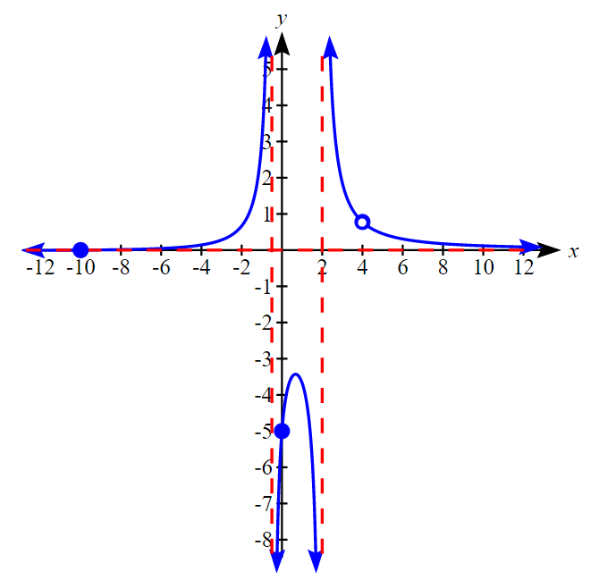.png?revision=1&size=bestfit&width=446&height=420)
We still need to find the range. Upon viewing the graph, we can see the range is not all real numbers so we will need to approximate the range using graphing technology. We can see there is a maximum within the interval \(\left(-\dfrac{1}{2},2\right)\). Using our graphing calculator, we find the maximum is \(\approx -3.428\).
Remember that there is is an x-intercept at \((-10,0)\). Although not easily viewable in the window used to sketch the graph in Figure \(\PageIndex{12}\), we know that they must be a local minimum within the interval \(\left(-\dfrac{1}{2},2\right)\). To approximate it using graphing technology you will need to find an appropriate window to view the local minimum so that you can then find it. The local minimum is \(\approx -0.012\). We can conclude from this that the range is \((-\infty,-3.428] \cup [-0.012,\infty)\).
One important thing to note about the graph of \(A(x)\). Most graphing viewing windows will not show the local minimum. It is important for hand drawn sketches to include this information. Also, this example also illustrates the importance of understanding how functions behave as we would have not known there was a local minimum within the interval \(\left(-\infty,-\dfrac{1}{2}\right)\) had we not investigated the behavior of the function.
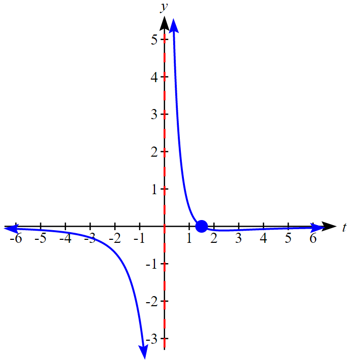
Find the asymptotes, intercepts, domain, and range of \(w(t)=\dfrac{3}{t}-\dfrac{3t+2}{t^2+1}\). Round to the third decimal place for the range, if applicable. Then, use this information to sketch \(w(t)\).
- Answer
-
Note that the function must be simplified before finding the graphical information we are asked to find. \[w(t)=\dfrac{3}{t}-\dfrac{3t+2}{t^2+1}=\dfrac{3-2t}{t(t^2+1)}\nonumber \]
The vertical asymptote is \(x=0\). The horizontal asymptote is \(y=0\).
There is a t-intercept at \((\dfrac{3}{2},0)\). This is the only intercept.
The domain is \((-\infty,0) \cup (0,\infty)\). The range is (\(-\infty,\infty)\). (note that there is a local minimum at \(\approx (2.382,-0.111)\).
Graph is shown in Figure \(\PageIndex{13}\).
.png?revision=1&size=bestfit&width=422&height=437)
Figure \(\PageIndex{13}\): Graph of w(t)
Finding Equations of Rational Functions that Model Graphical Information
Now that we have analyzed the equations for rational functions and how they relate to a graph of the function, we can use information given by a graph to write the function. A rational function written in factored form will have an x-intercept where each factor of the numerator is equal to zero. (An exception occurs in the case of a removable discontinuity.) As a result, we can form a numerator of a function whose graph will pass through a set of x-intercepts by introducing a corresponding set of factors. Likewise, because the function will have a vertical asymptote where each factor of the denominator is equal to zero, we can form a denominator that will produce the vertical asymptotes by introducing a corresponding set of factors.
Write an equation for the rational function shown in Figure \(\PageIndex{14}\).
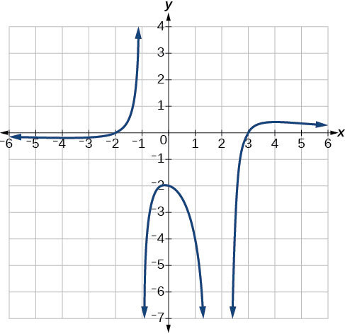
Solution
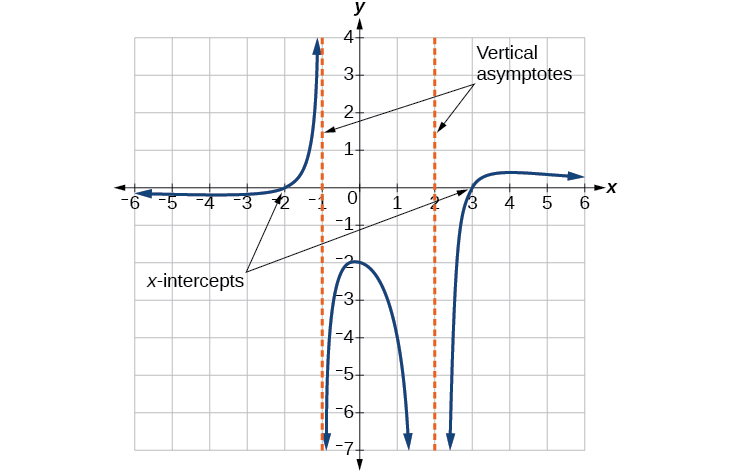
The graph appears to have x-intercepts at \(x=–2\) and \(x=3\). At both, the graph passes through the intercept, suggesting linear factors for the numerator. The graph has two vertical asymptotes at \(x=–1\) and \(x=2\) indicating denominator factors. Notice that at \(x=2\) that the graph approaches the asymptote from the same side. This indicates the factor \(x-2\) would be squared (think about what we know about sign charts and polynomial behavior). See Figure \(\PageIndex{15}\).
We can use this information to write a function of the form \[f(x)=a\dfrac{(x+2)(x−3)}{(x+1){(x−2)}^2}\nonumber\]
To find the stretch factor, \(a\), we can evaluate at a clear point on the graph, such as the y-intercept \((0,–2)\).
\[\begin{align*}−2&=a\dfrac{(0+2)(0−3)}{(0+1){(0−2)}^2} \\[6pt] -2&=a\left(\dfrac{−6}{4} \right) \\[6pt] a&=\dfrac{−8}{−6}=\dfrac{4}{3} \end{align*}\nonumber\]
This gives us a final function of \(f(x)=\dfrac{4(x+2)(x−3)}{3(x+1){(x−2)}^2}\).