5.3: Graphing Exponential Functions

Last updated
Save as PDF

Page ID: 89583

$ \newcommand{\vecs}[1]{\overset { \scriptstyle \rightharpoonup} {\mathbf{#1}} } $ $ \newcommand{\vecd}[1]{\overset{-\!-\!\rightharpoonup}{\vphantom{a}\smash {#1}}} $$\newcommand{\id}{\mathrm{id}}$ $ \newcommand{\Span}{\mathrm{span}}$ $ \newcommand{\kernel}{\mathrm{null}\,}$ $ \newcommand{\range}{\mathrm{range}\,}$ $ \newcommand{\RealPart}{\mathrm{Re}}$ $ \newcommand{\ImaginaryPart}{\mathrm{Im}}$ $ \newcommand{\Argument}{\mathrm{Arg}}$ $ \newcommand{\norm}[1]{\| #1 \|}$ $ \newcommand{\inner}[2]{\langle #1, #2 \rangle}$ $ \newcommand{\Span}{\mathrm{span}}$ $\newcommand{\id}{\mathrm{id}}$ $ \newcommand{\Span}{\mathrm{span}}$ $ \newcommand{\kernel}{\mathrm{null}\,}$ $ \newcommand{\range}{\mathrm{range}\,}$ $ \newcommand{\RealPart}{\mathrm{Re}}$ $ \newcommand{\ImaginaryPart}{\mathrm{Im}}$ $ \newcommand{\Argument}{\mathrm{Arg}}$ $ \newcommand{\norm}[1]{\| #1 \|}$ $ \newcommand{\inner}[2]{\langle #1, #2 \rangle}$ $ \newcommand{\Span}{\mathrm{span}}$$\newcommand{\AA}{\unicode[.8,0]{x212B}}$

Learning Objectives

Identify basic graphs of exponential functions and sketch their graphs.
Identify transformations of exponential functions.
Graph exponential functions.
Find equations of exponential functions that model graphical information.

Graphing Exponential Functions

Before we begin graphing, it is helpful to review the behavior of exponential growth. Recall the table of values for a function of the form $f(x)=b^x$ whose base is greater than one. We’ll use the function $f(x)=2^x$. Observe how the output values in Table $\PageIndex{1}$ change as the input increases by $1$.

Table $\PageIndex{1}$
$x$	$−3$	$−2$	$−1$	$0$	$1$	$2$	$3$
$f(x)=2^x$	$\dfrac{1}{8}$	$\dfrac{1}{4}$	$\dfrac{1}{2}$	$1$	$2$	$4$	$8$

Each output value is the product of the previous output and the base, $2$. We call the base $2$ the constant ratio. In fact, for any exponential function with the form $f(x)=ab^x$, $b$ is the constant ratio of the function. This means that as the input increases by $1$, the output value will be the product of the base and the previous output, regardless of the value of $a$.

Notice from the table that

the output values are positive for all values of $x$;
as $x$ increases, the output values increase without bound; and
as $x$ decreases, the output values grow smaller, approaching zero.

Figure $\PageIndex{1}$ shows the exponential growth function $f(x)=2^x$.

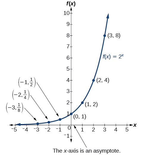
Graph of the exponential function, 2^(x), with labeled points at (-3, 1/8), (-2, ¼), (-1, ½), (0, 1), (1, 2), (2, 4), and (3, 8). The graph notes that the x-axis is an asymptote. — Figure $\PageIndex{1}$: Notice that the graph gets close to the x-axis, but never touches it.

The domain of $f(x)=2^x$ is all real numbers, the range is $(0,\infty)$, and the horizontal asymptote is $y=0$.

To get a sense of the behavior of exponential decay, we can create a table of values for a function of the form $f(x)=b^x$ whose base is between zero and one. We’ll use the function $g(x)={\left(\dfrac{1}{2}\right)}^x$. Observe how the output values in Table $\PageIndex{2}$ change as the input increases by $1$.

Table $\PageIndex{2}$
$x$	$-3$	$-2$	$-1$	$0$	$1$	$2$	$3$
$g(x)={\left(\dfrac{1}{2}\right)}^x$	$8$	$4$	$2$	$1$	$\dfrac{1}{2}$	$\dfrac{1}{4}$	$\dfrac{1}{8}$

Again, because the input is increasing by $1$, each output value is the product of the previous output and the base, or constant ratio $\dfrac{1}{2}$.

Notice from the table that

the output values are positive for all values of $x$;
as $x$ increases, the output values grow smaller, approaching zero; and
as $x$ decreases, the output values grow without bound.

Figure $\PageIndex{2}$ shows the exponential decay function, $g(x)={\left(\dfrac{1}{2}\right)}^x$.

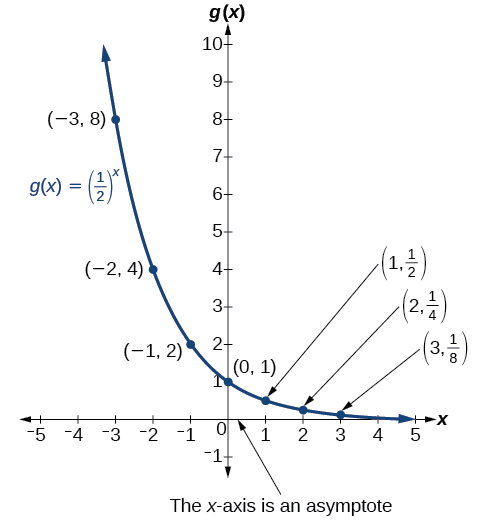
Graph of decreasing exponential function, (1/2)^x, with labeled points at (-3, 8), (-2, 4), (-1, 2), (0, 1), (1, 1/2), (2, 1/4), and (3, 1/8). The graph notes that the x-axis is an asymptote. — Figure $\PageIndex{2}$

The domain of $g(x)={\left(\dfrac{1}{2}\right)}^x$ is all real numbers, the range is $(0,\infty)$, and the horizontal asymptote is $y=0$.

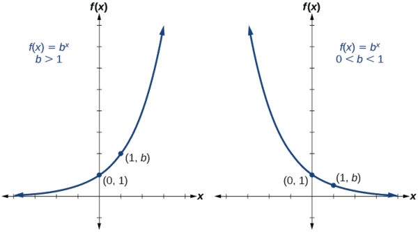
Characteristics of Basic Exponential Functions

An exponential function of the form $f(x)=b^x$, $b>0$, $b≠1$, has the following characteristics:

one-to-one function
horizontal asymptote: $y=0$
domain: $(–\infty, \infty)$
range: $(0,\infty)$
x-intercept: none
y-intercept: $(0,1)$
point at $(1,b)$
increasing if $b>1$
decreasing if $b<1$

Figure $\PageIndex{3}$ compares the graphs of exponential growth and decay functions.

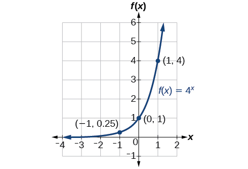
Graph of two functions where the first graph is of a function of f(x) = b^x when b>1 and the second graph is of the same function when b is 0<b<1. Both graphs have the points (0, 1) and (1, b) labeled. — Figure $\PageIndex{3}$

Example $\PageIndex{1}$

Sketch the graph of $f(x)=4^x$. State the domain, range, and asymptote.

Solution

Before graphing, identify the behavior and key points for the graph.

Since $b=4$ is greater than one, we know the function is increasing. The left tail of the graph will approach the horizontal asymptote, $y=0$, and the right tail will increase without bound.
The $y$-intercept is $(0,1)$.
The point $(1,4)$ is on the graph.
We draw and label the asymptote, plot and label the points, and draw a smooth curve through the points.

The domain is $(−\infty,\infty)$; the range is $(0,\infty)$; the horizontal asymptote is $y=0$.

$Graph of the increasing exponential function f(x) = 4^x with labeled points at (-1, 0.25), (0, 1), and (1, 4).$

To get a better feeling for the effect of $a$ and $b$ on the graph of $f(x)=ab^x$, examine the sets of graphs below. The first set shows various graphs, where $a$ remains the same and we only change the value for $b$.

$屏幕快照 2019-06-24 下午8.01.01.png$

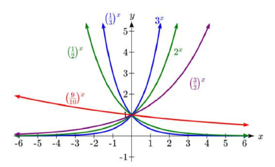
Notice that the closer the value of $b$ is to 1, the less steep the graph will be. The growth/decay is faster the further $b$ is from 1.

In the next set of graphs, $a$ is altered and our value for $b$ remains the same.

$屏幕快照 2019-06-24 下午8.02.55.png$

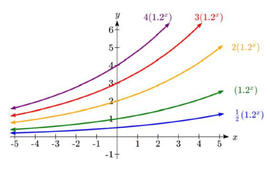
Notice that changing the value for $a$ changes the y-intercept. Since $a$ is multiplying the ${b}^{x}$ term, $a$ acts as a vertical stretch factor, not as a shift. Notice also that the end behavior for all of these functions is the same because the growth factor did not change and none of these $a$ values introduced a vertical flip.

Example $\PageIndex{2}$

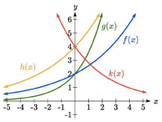
Match each equation with its graph. 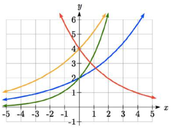$屏幕快照 2019-06-24 下午8.10.45.png$

\[{f(x)=2(1.3)^{x} }\nonumber\]

\[{g(x)=2(1.8)^{x} }\nonumber\]

\[{h(x)=4(1.3)^{x} }\nonumber\]

\[{k(x)=4(0.7)^{x} }\nonumber\]

Solution

The graph of $k(x)$ is the easiest to identify, since it is the only equation with a growth factor less than one, which will produce a decreasing graph. The graph of $h(x)$ can be identified as the only growing exponential function with a vertical intercept at (0,4). The graphs of $f(x)$ and $g(x)$ both have a vertical intercept at (0,2), but since $g(x)$ has a larger growth factor, we can identify it as the graph increasing faster.

$屏幕快照 2019-06-24 下午8.13.10.png$

Graphing Transformations of Exponential Functions

Transformations of exponential graphs behave similarly to those of other functions. Just as with other basic functions, we can apply the four types of transformations—shifts, reflections, stretches, and compressions—to the basic function $f(x)=b^x$ without loss of shape. For instance, just as the quadratic function maintains its parabolic shape when shifted, reflected, stretched, or compressed, the exponential function also maintains its general shape regardless of the transformations applied.

Graphing a Vertical Shift

The first transformation occurs when we add a constant $d$ to the basic function $f(x)=b^x$, giving us a vertical shiftd d units in the same direction as the sign. For example, if we begin by graphing a basic function, $f(x)=2^x$, we can then graph two vertical shifts alongside it, using $d=3$: the upward shift, $g(x)=2^x+3$ and the downward shift, $h(x)=2^x−3$. Both vertical shifts are shown in Figure $\PageIndex{4}$.

Graph of three functions, g(x) = 2^x+3 in blue with an asymptote at y=3, f(x) = 2^x in orange with an asymptote at y=0, and h(x)=2^x-3 with an asymptote at y=-3. Note that each functions’ transformations are described in the text. — Figure $\PageIndex{4}$

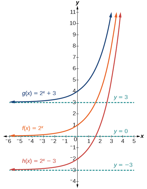
Observe the results of shifting $f(x)=2^x$ vertically:

The domain, $(−\infty,\infty)$ remains unchanged.
When the function is shifted up $3$ units to $g(x)=2^x+3$:
- The y-intercept shifts up $3$ units to $(0,4)$.
- The asymptote shifts up $3$ units to $y=3$.
- The range becomes $(3,\infty)$.
When the function is shifted down $3$ units to $h(x)=2^x−3$:
- The y-intercept shifts down $3$ units to $(0,−2)$.
- The asymptote also shifts down $3$ units to $y=−3$.
- The range becomes $(−3,\infty)$.

Graphing a Horizontal Shift

The next transformation occurs when we add a constant $c$ to the input of the basic function $f(x)=b^x$, giving us a horizontal shift $c$ units in the opposite direction of the sign. For example, if we begin by graphing the basic function $f(x)=2^x$, we can then graph two horizontal shifts alongside it, using $c=3$: the shift left, $g(x)=2^{x+3}$, and the shift right, $h(x)=2^{x−3}$. $h(x)=2^{x−3}$. Both horizontal shifts are shown in Figure $\PageIndex{5}$.

Graph of three functions, g(x) = 2^(x+3) in blue, f(x) = 2^x in orange, and h(x)=2^(x-3). Each functions’ asymptotes are at y=0Note that each functions’ transformations are described in the text. — Figure $\PageIndex{5}$

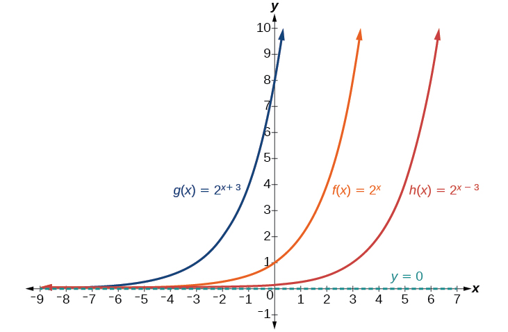
Observe the results of shifting $f(x)=2^x$ horizontally:

The domain, $(−\infty,\infty)$,remains unchanged.
The asymptote, $y=0$,remains unchanged.
The y-intercept shifts such that:
- When the function is shifted left $3$ units to $g(x)=2^{x+3}$, the y-intercept of the basic function shifts to (-3,1). The y-intercept of $g(x)$ is $(0,8)$ which can be found by evaluating the function at $x=0$.
- When the function is shifted right $3$ units to $h(x)=2^{x−3}$, the y-intercept of the basic function shifts to (3,1). The y-intercept of $h(x)$ is $(0,\dfrac{1}{8})$.

Example $\PageIndex{3}$

Identify the transformations and use them to sketch the graph of $f(x)=2^{x+1}−3$. State the domain, range, and asymptote.

Solution

We have an exponential equation of the form $f(x)=b^{x+c}+d$, with $b=2$, $c=1$, and $d=−3$.

The basic function is $y=2^x$. The graph will shift left 1 unit and down 3 units.

Shifting left 1 unit and down 3 units results in the y-intercept of the basic graph shifting to $(−1,−2)$. The point $(1,2)$ on the basic graph shifts to $(0,-1)$. The horizontal asymptote $y=−3$.

Using these key points, asymptote, and the shape of $f(x)=2^x$, shift the whole graph left $1$ units and down $3$ units.

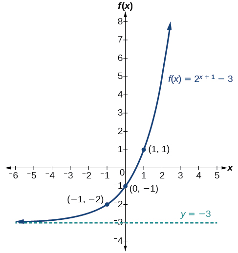
Graph of the function, f(x) = 2^(x+1)-3, with an asymptote at y=-3. Labeled points in the graph are (-1, -2), (0, -1), and (1, 1). — Figure $\PageIndex{6}$

The domain is $(−\infty,\infty)$; the range is $(−3,\infty)$; the horizontal asymptote is $y=−3$.

You Try $\PageIndex{1}$

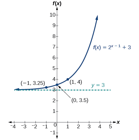
Identify the transformations and use them to sketch the graph of $f(x)=2^{x−1}+3$. State domain, range, and asymptote.

Answer

The basic function is $y=2^x$. The graph will shift right 1 unit and up 3 units.

The domain is $(−\infty,\infty)$; the range is $(3,\infty)$; the horizontal asymptote is $y=3$.

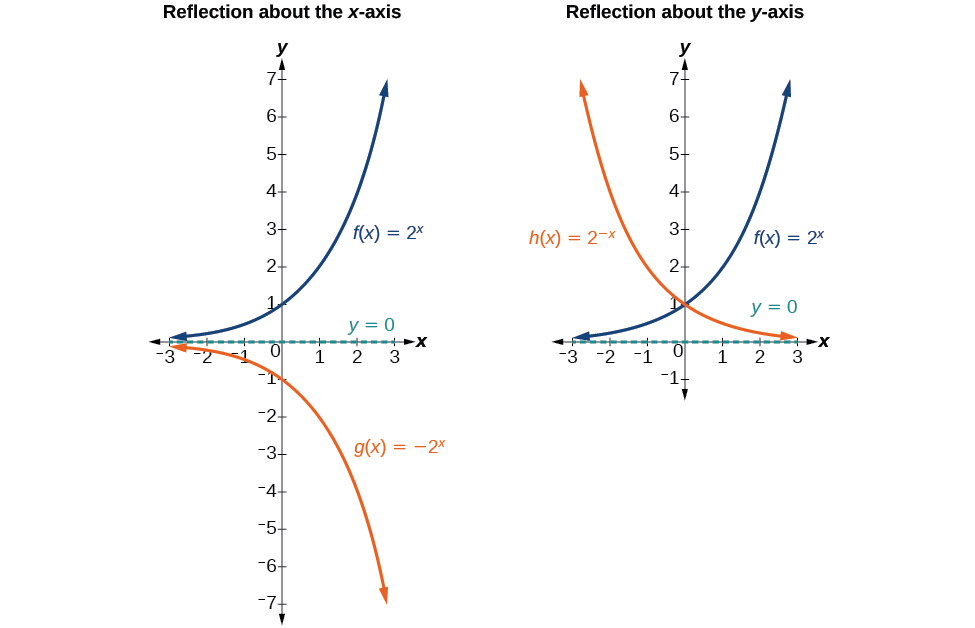
$Graph of the function, f(x) = 2^(x-1)+3, with an asymptote at y=3. Labeled points in the graph are (-1, 3.25), (0, 3.5), and (1, 4).$

Graphing Reflections

In addition to shifting, compressing, and stretching a graph, we can also reflect it about the x-axis or the y-axis. When we multiply the basic function $f(x)=b^x$ by $−1$, we get a reflection about the x-axis. When we multiply the input by $−1$, we get a reflection about the y-axis. The reflection about the x-axis, $g(x)=−2^x$, is shown on the left side of Figure $\PageIndex{7}$, and the reflection about the y-axis $h(x)=2^{−x}$, is shown on the right side of Figure $\PageIndex{7}$.

Two graphs where graph a is an example of a reflection about the x-axis and graph b is an example of a reflection about the y-axis. — Figure $\PageIndex{7}$: (a) $g(x)=−2^x$ reflects the graph of $f(x)=2^x$ about the x-axis. (b) $g(x)=2^{−x}$ reflects the graph of $f(x)=2^x$ about the y-axis.

Example $\PageIndex{4}$

Find and graph the equation for a function, $g(x)$, that reflects $f(x)={\left(\dfrac{1}{4}\right)}^x$ about the x-axis. State its domain, range, and asymptote.

Solution

Since we want to reflect the basic function $f(x)={\left(\dfrac{1}{4}\right)}^x$ about the x-axis, we multiply $f(x)$ by $−1$ to get, $g(x)=−{\left(\dfrac{1}{4}\right)}^x$. Next we create a table of points as in Table $\PageIndex{3}$.

Table $\PageIndex{3}$
$x$	$−3$	$−2$	$−1$	$0$	$1$	$2$	$3$
$g(x)=−{(\dfrac{1}{4})}^x$	$−64$	$−16$	$−4$	$−1$	$−0.25$	$−0.0625$	$−0.0156$

Plot the y-intercept, $(0,−1)$, along with two other points. We can use $(−1,−4)$ and $(1,−0.25)$.

Draw a smooth curve connecting the points:

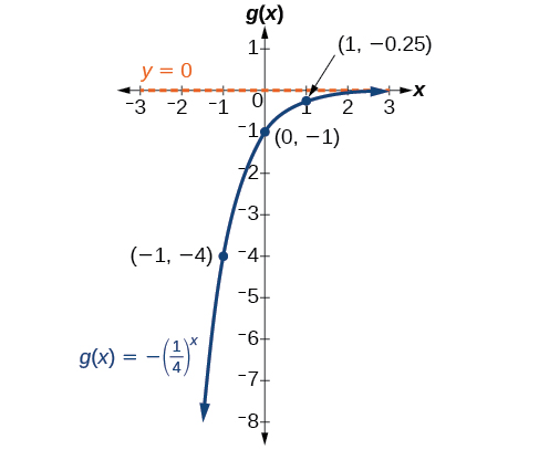
Graph of the function, g(x) = -(0.25)^(x), with an asymptote at y=0. Labeled points in the graph are (-1, -4), (0, -1), and (1, -0.25). — Figure $\PageIndex{8}$

The domain is $(−\infty,\infty)$; the range is $(−\infty,0)$; the horizontal asymptote is $y=0$.

Example $\PageIndex{5}$

Identify the transformations and use them to sketch the graph of $h(x)=3^{-x+2}-4$. State domain, range, and asymptote.

Solution

The basic function is $y=3^x$. Since $x$ is negative, we must first factor so we can identify the transformations. \[\begin{align*} f(x) &=3^{-x+2}-4 \\&= 3^{-(x-2)}-4\end{align*}\]

There is a y-axis reflection, a horizontal shift to the right 2 units, and a vertical shift down 4 units. The domain is $(−\infty,\infty)$; the range is $(0,\infty)$; the horizontal asymptote is $y=-4$.

Figure $\PageIndex{9}$: Graph of Transformed Exponential Function h(x).

You Try $\PageIndex{2}$

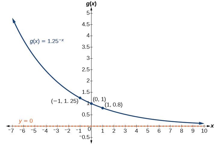
Find and graph the equation for a function, $g(x)$, that reflects $f(x)={1.25}^x$ about the y-axis. State its domain, range, and asymptote.

Answer

The equation of the reflected graph is $y=={1.25}^-x$; the domain is $(−\infty,\infty)$; the range is $(0,\infty)$; the horizontal asymptote is $y=0$.

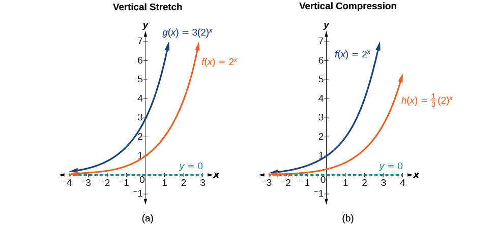
$Graph of the function, g(x) = -(1.25)^(-x), with an asymptote at y=0. Labeled points in the graph are (-1, 1.25), (0, 1), and (1, 0.8).$

Graphing a Stretch or Compression

While horizontal and vertical shifts involve adding constants to the input or to the function itself, a vertical stretch or compression occurs when we multiply the basic function $f(x)=b^x$ by a constant $|a|>0$. For example, if we begin by graphing the basic function $f(x)=2^x$,we can then graph the stretch, using $a=3$,to get $g(x)=3{(2)}^x$ as shown on the left in Figure $\PageIndex{10}$, and the compression, using $a=\dfrac{1}{3}$,to get $h(x)=\dfrac{1}{3}{(2)}^x$ as shown on the right in Figure $\PageIndex{10}$.

Two graphs where graph a is an example of vertical stretch and graph b is an example of vertical compression. — Figure $\PageIndex{10}$: (a) $g(x)=3{(2)}^x$ stretches the graph of $f(x)=2^x$ vertically by a factor of $3$. (b) $h(x)=\dfrac{1}{3}{(2)}^x$ compresses the graph of $f(x)=2^x$ vertically by a factor of $\dfrac{1}{3}$.

Example $\PageIndex{6}$

Sketch a graph of $f(x)=4{\left(\dfrac{1}{2}\right)}^x$. State the domain, range, and asymptote.

Solution

Before graphing, identify the behavior and key points on the graph.

Since $b=\dfrac{1}{2}$ this is a decreasing exponential function. The left end of the graph will increase without bound as $x$ decreases, and the right tail will approach the x-axis as $x$ increases.
Since $a=4$, the graph of $f(x)=4{\left(\dfrac{1}{2}\right)}^x$ will be stretched by a factor of $4$.

Create a table of points as shown in Table $\PageIndex{4}$.

Table $\PageIndex{4}$
$x$	$−3$	$−2$	$−1$	$0$	$1$	$2$	$3$
$f(x)=4{(\dfrac{1}{2})}^x$	$32$	$16$	$8$	$4$	$2$	$1$	$0.5$

Plot the y-intercept, $(0,4)$, along with two other points. We can use $(−1,8)$ and $(1,2)$. You may plot other points so your graph is more accurate also.

Draw a smooth curve connecting the points, as shown in Figure $\PageIndex{11}$.

Graph of the function, f(x) = 4(1/2)^(x), with an asymptote at y=0. Labeled points in the graph are (-1, 8), (0, 4), and (1, 2). — Figure $\PageIndex{11}$

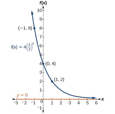
The domain is $(−\infty,\infty)$; the range is $(0,\infty)$; the horizontal asymptote is $y=0$.

You Try $\PageIndex{3}$

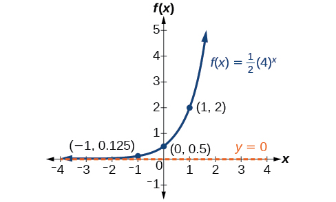
Sketch the graph of $f(x)=\dfrac{1}{2}{(4)}^x$. State the domain, range, and asymptote.

Answer

The domain is $(−\infty,\infty)$; the range is $(0,\infty)$; the horizontal asymptote is $y=0$.

$Graph of the function, f(x) = (1/2)(4)^(x), with an asymptote at y=0. Labeled points in the graph are (-1, 0.125), (0, 0.5), and (1, 2).$

Summary of Transformations of Exponential Functions

Now that we have worked with each type of transformation for the exponential function, we can summarize them to arrive at the general equation for translating exponential functions.

Transformations of Exponential Functions

A transformation of an exponential function has the form

$f(x)=ab^{x+c}+d$

where the basic function, $y=b^x$, $b>1$, is

shifted horizontally $c$ units to the left.
stretched vertically by a factor of $|a|$ if $|a|>0$.
compressed vertically by a factor of $|a|$ if $0<|a|<1$.
shifted vertically $d$ units.
reflected about the x-axis when $a<0$.

For $f(x)=b^{-x}$, the graph of the basic function is reflected about the y-axis.

Remember that the order for transformations follow the order of operations. This means that you start with stretch/compressions and reflections first, then shifts.

You Try $\PageIndex{4}$

What is the domain, range, asymptote, and end behavior of $y=8-e^{-x+7}$?

Answer: The domain is $(-\infty,\infty)$, the range is $(-\infty,8)$, the vertical asymptote is at $x=8$, as $x \rightarrow -\infty$, $y\rightarrow -\infty$, and as $x \rightarrow \infty$, $y\rightarrow 8$.

Finding Equations of Exponential Functions that Model Graphical Information

Example $\PageIndex{7}$

Write the equation for the function described below. Give the horizontal asymptote, the domain, and the range.

$f(x)=e^x$ is vertically stretched by a factor of $2$ , reflected across the y-axis, and then shifted up $4$ units.

Solution

We want to find an equation of the general form $f(x)=ab^{x+c}+d$. We use the description provided to find a, b, c, and d.

We are given the basic function $f(x)=e^x$, so $b=e$.
The function is stretched by a factor of $2$, so $a=2$.
There is no horizontal shift so $c=0$.
The function is reflected about the y-axis. We replace $x$ with $−x$ to get: $e^{−x}$.
The graph is shifted vertically 4 units, so $d=4$.

Substituting in the general form we get,

$f(x)=ab^{x+c}+d$

$=2e^{−x+0}+4$

$=2e^{−x}+4$

The domain is $(−\infty,\infty)$; the range is $(4,\infty)$; the horizontal asymptote is $y=4$.

You Try $\PageIndex{5}$

Write the equation for function described below. Give the horizontal asymptote, the domain, and the range.

$f(x)=e^x$ is compressed vertically by a factor of $\dfrac{1}{3}$, reflected across the x-axis and then shifted down $2$ units.

Answer: $f(x)=−\dfrac{1}{3}e^{x}−2$; the domain is $(−\infty,\infty)$; the range is $(−\infty,2)$; the horizontal asymptote is $y=2$.

Example $\PageIndex{8}$

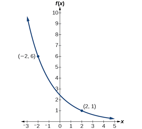
Find an exponential function that passes through the points $(−2,6)$ and $(2,1)$. Round to the nearest fourth decimal place.

Solution

Because we are not given the base for the function, we substitute both points into an equation of the form $f(x)=ab^x$, and then solve the system for $a$ and $b$.

Substituting $(−2,6)$ gives $6=ab^{−2}$
Substituting $(2,1)$ gives $1=ab^2$

Use the first equation to solve for $a$ in terms of $b$:

\[\begin{align*} 6&= ab^{-2}\\ 6&=\dfrac{a}{b^2} \qquad \text{Use properties of exponents to rewrite with positive expoents}\\ 6b^2&= a \qquad \text{Multiply by common denominator} \end{align*}\]

Substitute a in the second equation, and solve for $b$:

\[\begin{align*} 1&= ab^{2}\\ 1&= 6b^2 b^2 \qquad \text{Substitute a} \\ 1&= 6b^4 \qquad \text{Now, solve for b} \\ \dfrac{1}{6} &= b^4 \\ \left(\dfrac{1}{6}\right )^\frac{1}{4} &= \left(b^4\right)^\frac{1}{4} \\ b&= \left (\dfrac{1}{6} \right )^{\frac{1}{4}} \qquad \text{Round 4 decimal places rewrite the denominator}\\ b&\approx 0.6389 \end{align*}\]

Use the value of $b$ in the first equation to solve for the value of $a$:

\[\begin{align*} a&= 6b^{2}\\ &\approx 6(0.6389)^2 \\ &\approx 2.4492 \end{align*}\]

Thus, the equation is $f(x)=2.4492{(0.6389)}^x$.

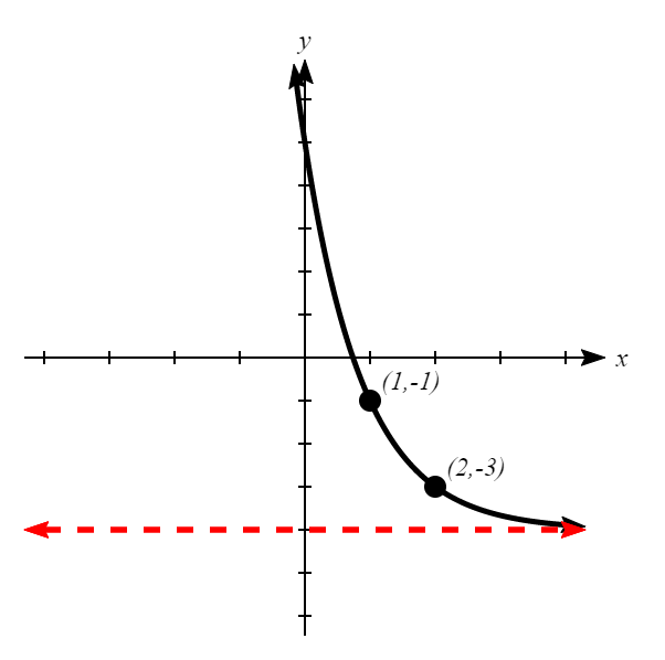
We can graph our model to check our work. Notice that the graph in Figure $\PageIndex{12}$ passes through the initial points given in the problem, $(−2, 6)$ and $(2, 1)$. The graph is an example of an exponential decay function.

Graph of the exponential function, f(x)=2.4492(0.6389)^x, with labeled points at (-2, 6) and (2, 1). — Figure $\PageIndex{12}$: The graph of $f(x)=2.4492{(0.6389)}^x$ models exponential decay.

You Try $\PageIndex{6}$

Given the two points $(1,3)$ and $(2,4.5)$, find the equation of the exponential function that passes through these two points.

Answer: $f(x)=2{(1.5)}^x$

\(x\)	\(−3\)	\(−2\)	\(−1\)	\(0\)	\(1\)	\(2\)	\(3\)
\(f(x)=2^x\)	\(\dfrac{1}{8}\)	\(\dfrac{1}{4}\)	\(\dfrac{1}{2}\)	\(1\)	\(2\)	\(4\)	\(8\)

\(x\)	\(-3\)	\(-2\)	\(-1\)	\(0\)	\(1\)	\(2\)	\(3\)
\(g(x)={\left(\dfrac{1}{2}\right)}^x\)	\(8\)	\(4\)	\(2\)	\(1\)	\(\dfrac{1}{2}\)	\(\dfrac{1}{4}\)	\(\dfrac{1}{8}\)

\(x\)	\(−3\)	\(−2\)	\(−1\)	\(0\)	\(1\)	\(2\)	\(3\)
\(g(x)=−{(\dfrac{1}{4})}^x\)	\(−64\)	\(−16\)	\(−4\)	\(−1\)	\(−0.25\)	\(−0.0625\)	\(−0.0156\)

\(x\)	\(−3\)	\(−2\)	\(−1\)	\(0\)	\(1\)	\(2\)	\(3\)
\(f(x)=4{(\dfrac{1}{2})}^x\)	\(32\)	\(16\)	\(8\)	\(4\)	\(2\)	\(1\)	\(0.5\)

Search

Characteristics of Basic Exponential Functions

Example \(\PageIndex{1}\)

Example \(\PageIndex{2}\)

Example \(\PageIndex{3}\)

You Try \(\PageIndex{1}\)

Example \(\PageIndex{4}\)

Example \(\PageIndex{5}\)

You Try \(\PageIndex{2}\)

Example \(\PageIndex{6}\)

You Try \(\PageIndex{3}\)

Transformations of Exponential Functions

You Try \(\PageIndex{4}\)

Example \(\PageIndex{7}\)

You Try \(\PageIndex{5}\)

Example \(\PageIndex{8}\)

You Try \(\PageIndex{6}\)