1.1: Graphing Equations by Hand

Last updated
Save as PDF

Page ID: 54948

$ \newcommand{\vecs}[1]{\overset { \scriptstyle \rightharpoonup} {\mathbf{#1}} } $ $ \newcommand{\vecd}[1]{\overset{-\!-\!\rightharpoonup}{\vphantom{a}\smash {#1}}} $$\newcommand{\id}{\mathrm{id}}$ $ \newcommand{\Span}{\mathrm{span}}$ $ \newcommand{\kernel}{\mathrm{null}\,}$ $ \newcommand{\range}{\mathrm{range}\,}$ $ \newcommand{\RealPart}{\mathrm{Re}}$ $ \newcommand{\ImaginaryPart}{\mathrm{Im}}$ $ \newcommand{\Argument}{\mathrm{Arg}}$ $ \newcommand{\norm}[1]{\| #1 \|}$ $ \newcommand{\inner}[2]{\langle #1, #2 \rangle}$ $ \newcommand{\Span}{\mathrm{span}}$ $\newcommand{\id}{\mathrm{id}}$ $ \newcommand{\Span}{\mathrm{span}}$ $ \newcommand{\kernel}{\mathrm{null}\,}$ $ \newcommand{\range}{\mathrm{range}\,}$ $ \newcommand{\RealPart}{\mathrm{Re}}$ $ \newcommand{\ImaginaryPart}{\mathrm{Im}}$ $ \newcommand{\Argument}{\mathrm{Arg}}$ $ \newcommand{\norm}[1]{\| #1 \|}$ $ \newcommand{\inner}[2]{\langle #1, #2 \rangle}$ $ \newcommand{\Span}{\mathrm{span}}$$\newcommand{\AA}{\unicode[.8,0]{x212B}}$

We begin with the deﬁnition of an ordered pair.

Ordered Pair

The construct $(x,y)$, where $x$ and $y$ are any real numbers, is called an ordered pair of real numbers.

$(4,3)$, $(−3,4)$, $(−2,−3)$, and $(3,−1)$ are examples of ordered pairs.

Order Matters

Pay particular attention to the phrase “ordered pairs.” Order matters. Consequently, the ordered pair $(x,y)$ is not the same as the ordered pair $(y,x)$, because the numbers are presented in a diﬀerent order.

The Cartesian Coordinate System

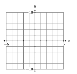
Pictured in Figure $\PageIndex{1}$ is a Cartesian Coordinate System. On a grid, we’ve created two real lines, one horizontal labeled $x$ (we’ll refer to this one as the $x$-axis), and the other vertical labeled $y$ (we’ll refer to this one as the $y$-axis).

fig 3.1.1.png — Figure $\PageIndex{1}$: The Cartesian Coordinate System.

Two Important Points:

Here are two important points to be made about the horizontal and vertical axes in Figure $\PageIndex{1}$.

As you move from left to right along the horizontal axis (the $x$-axis in Figure $\PageIndex{1}$), the numbers grow larger. The positive direction is to the right, the negative direction is to the left.
As you move from bottom to top along the vertical axis (the $y$-axis in Figure $\PageIndex{1}$), the numbers grow larger. The positive direction is upward, the negative direction is downward.

Additional Comments:

fig 3.1.2.png — Figure $\PageIndex{2}$: Numbering the quadrants and indicating the coordinates of the origin.

Two additional comments are in order:

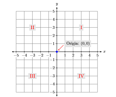
The point where the horizontal and vertical axes intersect in Figure $\PageIndex{2}$ is called the origin of the coordinate system. The origin has coordinates $(0,0)$.
The horizontal and vertical axes divide the plane into four quadrants, numbered $\mathrm{I}, \mathrm{II}, \mathrm{MI},$ and $\mathrm{IV}$ (roman numerals for one, two, three, and four), as shown in Figure $\PageIndex{2}$. Note that the quadrants are numbered in a counter-clockwise order.

Note

Rene Descartes (1596-1650) was a French philosopher and mathematician who is well known for the famous phrase“cogito ergo sum” (I think, therefore I am), which appears in his Discours de la methode pour bien conduire sa raison, et chercher la verite dans les sciences (Discourse on the Method of Rightly Conducting the Reason, and Seeking Truth in the Sciences). In that same treatise, Descartes introduces his coordinate system, a method for representing points in the plane via pairs of real numbers. Indeed, the Cartesian plane of modern day is so named in honor of Rene Descartes, who some call the “Father of Modern Mathematics”

Plotting Ordered Pairs

Before we can plot any points or draw any graphs, we ﬁrst need to set up a Cartesian Coordinate System on a sheet of graph paper? How do we do this? What is required?

how to setup cartesian coordinate system

Draw and label each axis.

If we are going to plot points (x,y), then, on a sheet of graph paper, perform each of the following initial tasks.

Use a ruler to draw the horizontal and vertical axes.
Label the horizontal axis as the $x$-axis and the vertical axis as the $y$-axis.

We don’t always label the horizontal axis as the $x$-axis and the vertical axis as the $y$-axis. For example, if we want to plot the velocity of an object as a function of time, then we would be plotting points $(t,v)$. In that case, we would label the horizontal axis as the $t$-axis and the vertical axis as the $v$-axis.

Indicate the scale on each axis.

Label at least one vertical gridline with its numerical value.
Label at least one horizontal gridline with its numerical value.

The scales on the horizontal and vertical axes may diﬀer. However, on each axis, the scale must remain consistent. That is, as you count to the right from the origin on the $x$-axis, if each gridline represents one unit, then as you count to the left from the origin on the $x$-axis, each gridline must also represent one unit. Similar comments are in order for the $y$-axis, where the scale must also be consistent, whether you are counting up or down.

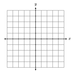
The result of this ﬁrst step is shown in Figure $\PageIndex{3}$.

fig 3.1.3.png — Figure $\PageIndex{3}$: Draw and label each axis.

An example is shown in Figure $\PageIndex{4}$. Note that the scale indicated on the $x$-axis indicates that each gridline counts as $1$-unit as we count from left-to-right. The scale on the $y$-axis indicates that each gridlines counts as $2$-units as we count from bottom-to-top.

fig 3.1.4.png — Figure $\PageIndex{4}$: Indicate the scale on each axis.

Now that we know how to set up a Cartesian Coordinate System on a sheet of graph paper, here are two examples of how we plot points on our coordinate system.

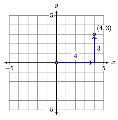
To plot the ordered pair $(4,3)$, start at the origin and move $4$ units to the right along the horizontal axis, then $3$ units upward in the direction of the vertical axis.

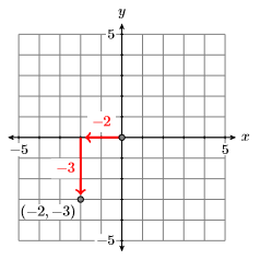
fig 3.1.5.png — Figure $\PageIndex{5}$: Plot of $(4,3)$.

To plot the ordered pair $(−2,−3)$, start at the origin and move $2$ units to the left along the horizontal axis, then $3$ units downward in the direction of the vertical axis.

fig 3.1.6.png — Figure $\PageIndex{6}$: Plot of $(-2,-3)$

Continuing in this manner, each ordered pair $(x,y)$ of real numbers is associated with a unique point in the Cartesian plane. Vice-versa, each point in the Cartesian point is associated with a unique ordered pair of real numbers. Because of this association, we begin to use the words “point” and “ordered pair” as equivalent expressions, sometimes referring to the “point” $(x,y)$ and other times to the “ordered pair” $(x,y)$.

Example $\PageIndex{1}$

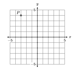
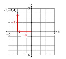
Identify the coordinates of the point $P$ in Figure $\PageIndex{7}$.

fig 3.1.7.png — Figure $\PageIndex{7}$: Identify the coordinates of the point $P$.

Solution

In Figure $\PageIndex{8}$, start at the origin, move $3$ units to the left and $4$ units up to reach the point $P$. This indicates that the coordinates of the point $P$ are $(−3,4)$.

fig 3.1.8.png — Figure $\PageIndex{8}$: Start at the origin, move $3$ units left and $4$ units up.

Exercise $\PageIndex{1}$

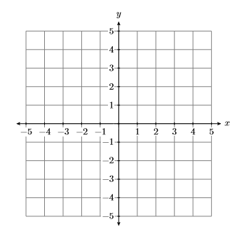
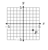
Identify the coordinates of the point $P$ in the graph below.

$Exercise 3.1.1.png$

Answer: $(3,-2)$

Equations in Two Variables

Note

The variables do not have to always be $x$ and $y$. For example, the equation $v =2+3 .2t$ is an equation in two variables, $v$ and $t$.

The equation $y = x + 1$ is an equation in two variables, in this case $x$ and $y$. Consider the point $(x,y) = (2 ,3)$. If we substitute $2$ for $x$ and $3$ for $y$ in the equation $y = x + 1$, we get the following result:

\[\begin{aligned} y &= x+1 \quad \color {Red} \text { Original equation. } \\ 3 &= 2+1 \quad \color {Red} \text { Substitute: } 2 \text { for } x, 3 \text { for } y \\ 3 &= 3 \quad \color {Red} \text { Simplify both sides. } \end{aligned} \nonumber \]

Because the last line is a true statement, we say that $(2,3)$ is a solution of the equation $y = x + 1$. Alternately, we say that $(2,3)$ satisﬁes the equation $y = x + 1$. On the other hand, consider the point $(x,y)=(−3,1)$. If we substitute $−3$ for $x$ and $1$ for $y$ in the equation $y = x + 1$, we get the following result.

\[\begin{aligned} y &= x+1 \quad \color {Red} \text { Original equation. } \\ 1 &= -3+1 \quad \color {Red} \text { Substitute: } -3 \text { for } x, 1 \text { for } y \\ 1 &= -2 \quad \color {Red} \text { Simplify both sides. } \end{aligned} \nonumber \]

Because the last line is a false statement, the point $(−3,1)$ is not a solution of the equation $y = x+1$; that is, the point $(−3,1)$ does not satisfy the equation $y = x + 1$.

Solutions of an equation in two variables

Given an equation in the variables $x$ and $y$ and a point $(x,y)=(a,b)$, if upon subsituting $a$ for $x$ and $b$ for $y$ a true statement results, then the point $(x,y)=(a,b)$ is said to be a solution of the given equation. Alternately, we say that the point $(x,y)=(a,b)$ satisﬁes the given equation.

Example $\PageIndex{2}$

Which of the ordered pairs $(0,−3)$ and $(1,1)$ satisfy the equation $y =3x−2$?

Solution

Substituting the ordered pairs $(0,−3)$ and $(1,1)$ into the equation $y =3x−2$ lead to the following results:

Consider $(x,y) = (0 ,−3)$. Substitute $0$ for $x$ and $−3$ for $y$:

\[\begin{aligned} y &=3 x-2 \\-3 &=3(0)-2 \\-3 &=-2 \end{aligned} \nonumber \]

The resulting statement is false.

Consider $(x,y) = (1 ,1)$. Substitute $1$ for $x$ and $1$ for $y$:

\[\begin{aligned} y &=3x-2 \\ 1 &=3(1)-2 \\ 1 &=1 \end{aligned} \nonumber\]

The resulting statement is true.

Thus, the ordered pair $(0,−3)$ does not satisfy the equation $y =3 x−2$, but the ordered pair $(1 ,1)$ does satisfy the equation $y =3x−2$.

Exercise $\PageIndex{2}$

Which of the ordered pairs $(−1,3)$ and $(2,1)$ satisfy the equation $y =2x + 5$?

Answer: $(-1,3)$

Graphing Equations in Two Variables

Let’s ﬁrst deﬁne what is meant by the graph of an equation in two variables.

The graph of an equation

The graph of an equation is the set of all points that satisfy the given equation.

Example $\PageIndex{3}$

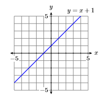
Sketch the graph of the equation $y = x + 1$.

Solution

The deﬁnition requires that we plot all points in the Cartesian Coordinate System that satisfy the equation $y = x + 1$. Let’s ﬁrst create a table of points that satisfy the equation. Start by creating three columns with headers $x$, $y$, and $(x,y)$, then select some values for $x$ and put them in the ﬁrst column.

Take the ﬁrst value of $x$, namely $x = −3$, and substitute it into the equation $y = x + 1$.

\[\begin{aligned}y &=x+1 \\ y &=-3+1 \\ y &=-2\end{aligned} \nonumber \]

\[\begin{array}{|c|c|c|c|}\hline x & {y=x+1} & {(x, y)} \\ \hline-3 & {-2} & {(-3,-2)} \\ -2 & {} & {} \\ {-1} & {} & {} \\ { 0} & {} & {}\\ {1} & {} & {}\\ {2} & {} & {}\\ {3} & {} &{} \\ \hline\end{array} \nonumber \]

Thus, when $x = −3$, we have $y = −2$. Enter this value into the table.

Continue substituting each tabular value of $x$ into the equation $y = x + 1$ and use each result to complete the corresponding entries in the table.

\[\begin{array}{l}{y=-3+1=-2} \\ {y=-2+1=-1} \\ {y=-1+1=0} \\ {y=0+1=1} \\ {y=1+1=2} \\ {y=2+1=3} \\ {y=3+1=4}\end{array} \nonumber \]

\[\begin{array}{|c|c|c|c|}\hline x & {y=x+1} & {(x, y)} \\ \hline-3 & {-2} & {(-3,-2)} \\ -2 & {-1} & {(-2,-1)} \\ {-1} & {0} & {(-1,0)} \\ { 0} & {1} & {(0,1)}\\ {1} & {2} & {(1,2)}\\ {2} & {3} & {(2,3)}\\ {3} & {4} &{(3,4)} \\ \hline\end{array} \nonumber \]

The last column of the table now contains seven points that satisfy the equation $y = x+1$. Plot these points on a Cartesian Coordinate System (see Figure $\PageIndex{9}$).

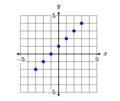
fig 3.1.9.png — Figure $\PageIndex{9}$: Seven points that satisfy the equation $y = x + 1$.

In Figure $\PageIndex{9}$, we have plotted seven points that satisfy the given equation $y = x+1$. However, the deﬁnition requires that we plot all points that satisfy the equation. It appears that a pattern is developing in Figure $\PageIndex{9}$, but let’s calculate and plot a few more points in order to be sure. Add the $x$-values $−2.5$, $−1.5$, $−0.5$, $0.5$, $1.5$, and $2.5$ to the x-column of the table, then use the equation $y = x + 1$ to evaluate y at each one of these $x$-values.

\[\begin{array}{l}{y=-2.5+1=-1.5} \\ {y=-1.5+1=-0.5} \\ {y=-0.5+1=0.5} \\ {y=0.5+1=1.5} \\ {y=1.5+1=2.5} \\ {y=2.5+1=3.5}\end{array} \nonumber \]

\[\begin{array}{|c|c|c|c|}\hline x & {y=x+1} & {(x, y)} \\ \hline-2.5 & {-1.5} & {(-2.5,-1.5)} \\ -1.5 & {-0.5} & {(-1.5,-0.5)} \\ {-0.5} & {0.5} & {(-0.5,0.5)} \\ { 0.5} & {1.5} & {(0.5,1.5)}\\ {1.5} & {2.5} & {(1.5,2.5)}\\ {2.5} & {3.5} & {(2.5,3.5)}\\ \hline\end{array} \nonumber \]

Add these additional points to the graph in Figure $\PageIndex{9}$ to produce the image shown in Figure $\PageIndex{10}$.

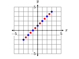
fig 3.1.10.png — Figure $\PageIndex{10}$: Adding additional points to the graph of $y = x + 1$.

There are an inﬁnite number of points that satisfy the equation $y = x + 1$. In Figure $\PageIndex{10}$, we’ve plotted only $13$ points that satisfy the equation. However, the collection of points plotted in Figure $\PageIndex{10}$ suggest that if we were to plot the remainder of the points that satisfy the equation $y = x + 1$, we would get the graph of the line shown in Figure $\PageIndex{11}$.

fig 3.1.11.png — Figure $\PageIndex{11}$: The graph of $y = x + 1$ is a line.

Exercise $\PageIndex{3}$

Sketch the graph of the equation $y = −x + 2$.

Answer: $Exercise 3.1.3.png$

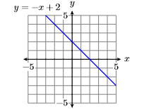
Guidelines and Requirements

Example $\PageIndex{3}$ suggests that we should use the following guidelines when sketching the graph of an equation.

Guidelines for drawing the graph of an equation

When asked to draw the graph of an equation, perform each of the following steps:

Set up and calculate a table of points that satisfy the given equation.
Set up a Cartesian Coordinate System on graph paper and plot the points in your table on the system. Label each axis (usually $x$ and $y$) and indicate the scale on each axis.
If the number of points plotted are enough to envision what the shape of the ﬁnal curve will be, then draw the remaining points that satisfy the equation as imagined. Use a ruler if you believe the graph is a line. If the graph appears to be a curve, freehand the graph without the use of a ruler.
If the number of plotted points do not provide enough evidence to envision the ﬁnal shape of the graph, add more points to your table, plot them, and try again to envision the ﬁnal shape of the graph. If you still cannot predict the eventual shape of the graph, keep adding points to your table and plotting them until you are convinced of the ﬁnal shape of the graph.

Here are some additional requirements that must be followed when sketching the graph of an equation.

Graph paper, lines, curves, and rulers.

The following are requirements for this class:

All graphs are to be drawn on graph paper.
All lines are to be drawn with a ruler. This includes the horizontal and vertical axes.
If the graph of an equation is a curve instead of a line, then the graph should be drawn freehand, without the aid of a ruler.

Using the TABLE Feature of the Graphing Calculator

As the equations become more complicated, it can become quite tedious to create tables of points that satisfy the equation. Fortunately, the graphing calculator has a TABLE feature that enables you to easily construct tables of points that satisfy the given equation.

Example $\PageIndex{4}$

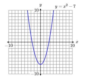
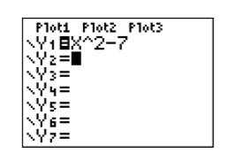
Use the graphing calculator to help create a table of points that satisfy the equation $y = x^2−7$. Plot the points in your table. If you don’t feel that there is enough evidence to envision what the ﬁnal shape of the graph will be, use the calculator to add more points to your table and plot them. Continue this process until your are convinced of the ﬁnal shape of the graph.

Solution

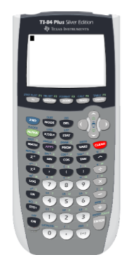
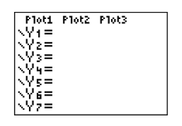
fig 3.1.12.png — Figure $\PageIndex{12}$: The graphing calculator.

The ﬁrst step is to load the equation $y = x^2−7$ into the Y= menu of the graphing calculator. The topmost row of buttons on your calculator (see Figure $\PageIndex{12}$) have the following appearance:

fig 3.1.a.png — Figure $\PageIndex{13}$. Use the up-and-down arrow keys (see Figure $\PageIndex{15}$) to move the cursor after Y1= in the Y= menu, then use the following keystrokes to enter the equation $y = x^2 −7$. The result is shown in Figure $\PageIndex{14}$.

$fig 3.1.b.png$

fig 3.1.13.png — Figure $\PageIndex{13}$: Opening the Y= menu. **Figure** **$\PageIndex{14}$**: Entering the equation $y = x^2 −7$.

alt — Figure $\PageIndex{13}$: Opening the Y= menu. **Figure** **$\PageIndex{14}$**: Entering the equation $y = x^2 −7$.

fig 3.1.15.png — Figure $\PageIndex{15}$: Arrow keys move the cursor.

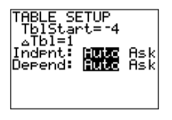
The next step is to “set up” the table. First, note that the calculator has symbolism printed on its case above each of its buttons. Above the WINDOW button you’ll note the phrase TBLSET. Note that it is in the same color as the 2ND button. Thus, to open the setup window for the table, enter the following keystrokes.

alt — Figure $\PageIndex{16}$) equal to the ﬁrst x-value you want to see in your table. In this case, enter $−4$ after TblStart. SetTbl to the increment you want for your $x$-values. In this case, set Tbl equal to $1$. Finally, set both the independent and dependent variables to “automatic.” In each case, use the arrow keys to highlight the word AUTO and press ENTER. The result is shown in Figure $\PageIndex{16}$.

fig 3.1.c.png — Figure $\PageIndex{16}$) equal to the ﬁrst x-value you want to see in your table. In this case, enter $−4$ after TblStart. SetTbl to the increment you want for your $x$-values. In this case, set Tbl equal to $1$. Finally, set both the independent and dependent variables to “automatic.” In each case, use the arrow keys to highlight the word AUTO and press ENTER. The result is shown in Figure $\PageIndex{16}$.

Next, note the word TABLE above the GRAPH button is in the same color as the 2ND key. To open the TABLE, enter the following keystrokes.

fig 3.1.d.png — Figure $\PageIndex{17}$. Note that you can use the up-and-down arrow keys to scroll through the table.

fig 3.1.16.png — Figure $\PageIndex{16}$: Opening the TBLSET menu. **Figure $\PageIndex{17}$**: Table of points satisfying $y = x^2 −7$.

fig 3.1.17.png — Figure $\PageIndex{16}$: Opening the TBLSET menu. **Figure $\PageIndex{17}$**: Table of points satisfying $y = x^2 −7$.

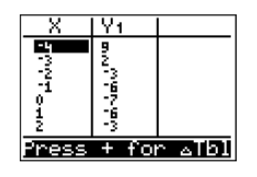
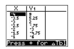
Next, enter the results from your calculator’s table into a table on a sheet of graph paper, then plot the points in the table. The results are shown in Figure $\PageIndex{18}$.

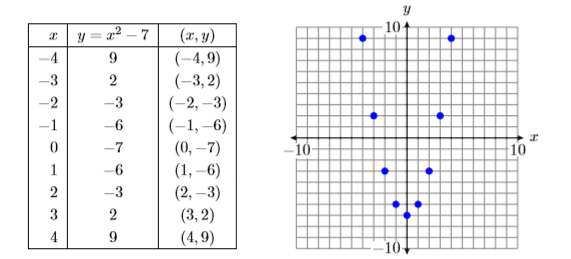
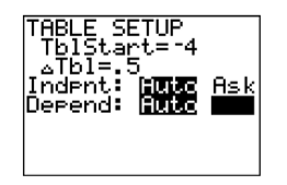
fig 3.1.18.png — Figure $\PageIndex{18}$: Plotting nine points that satisfy the equation $y = x^2 −7$.

In Figure $\PageIndex{18}$, the eventual shape of the graph of $y = x^2 −7$ may be evident already, but let’s add a few more points to our table and plot them. Open the table “setup” window again by pressing 2ND WINDOW. Set TblStart to $−4$ again, then set the increment Tbl to $0.5$. The result is shown in Figure $\PageIndex{19}$.

fig 3.1.19.png — Figure $\PageIndex{19}$: SetTbl equal to 0.5. **Figure $\PageIndex{20}$:** More points satisfying $y = x^2 −7$.

fig 3.1.20.png — Figure $\PageIndex{19}$: SetTbl equal to 0.5. **Figure $\PageIndex{20}$:** More points satisfying $y = x^2 −7$.

Add these new points to the table on your graph paper and plot them (see Figure $\PageIndex{21}$).

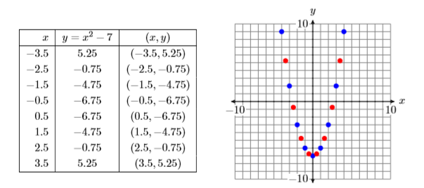
fig 3.1.21.png — Figure $\PageIndex{21}$: Adding additional points to the graph of $y = x^2 −7$.

There are an inﬁnite number of points that satisfy the equation $y = x^2−7$. In Figure $\PageIndex{21}$, we’ve plotted only $17$ points that satisfy the equation $y = x^2 −7$. However, the collection of points in Figure $\PageIndex{21}$ suggest that if we were to plot the remainder of the points that satisfy the equation $y = x^2 −7$, the result would be the curve (called a parabola) shown in Figure $\PageIndex{22}$.