2.6: Extrema and Models

In the last section, we used end-behavior and zeros to sketch the graph of a given polynomial. We also mentioned that it takes a semester of calculus to learn an analytic technique used to calculate the “turning points” of the polynomial. That said, we’ll still pursue the coordinates of the “turning points” in this section, but we will use the graphing calculator to assist us in this quest; and then we will use this technique with some applications.

Extrema

Before we begin, we’d first like to differentiate between local extrema and absolute extrema. This is best accomplished by means of an example. Consider, if you will, the graphs of three polynomial functions in Figure 1.

In the first figure, Figure \(\PageIndex{1a}\), the point A is the “absolute” lowest point on the graph. Therefore, the y-value of point A is an absolute minimum value of the function.

In the second figure, Figure \(\PageIndex{1b}\), there is no “absolute” highest point on the graph (the graph goes up to positive infinity), nor is there an “absolute” lowest point on the graph (the graph goes down to negative infinity). Therefore, this function has neither an absolute minimum nor an absolute maximum.

However, point B in Figure \(\PageIndex{1b}\) is the highest point in its immediate neighborhood. If you wander too far to the right, there are points on the graph higher than point B, but locally point B is the highest point. Therefore, the y-value of point B is called a local maximum value of the function.

Similarly, point C in Figure \(\PageIndex{1b}\) is the lowest point in its immediate neighborhood. If you wander too far to the left, there are points on the graph lower than point C, but, in its neighborhood, point C is the lowest point. Therefore, the y-value of point C is called a local minimum of the function.

Figure \(\PageIndex{1}\): Differentiating between local and absolute extrema.

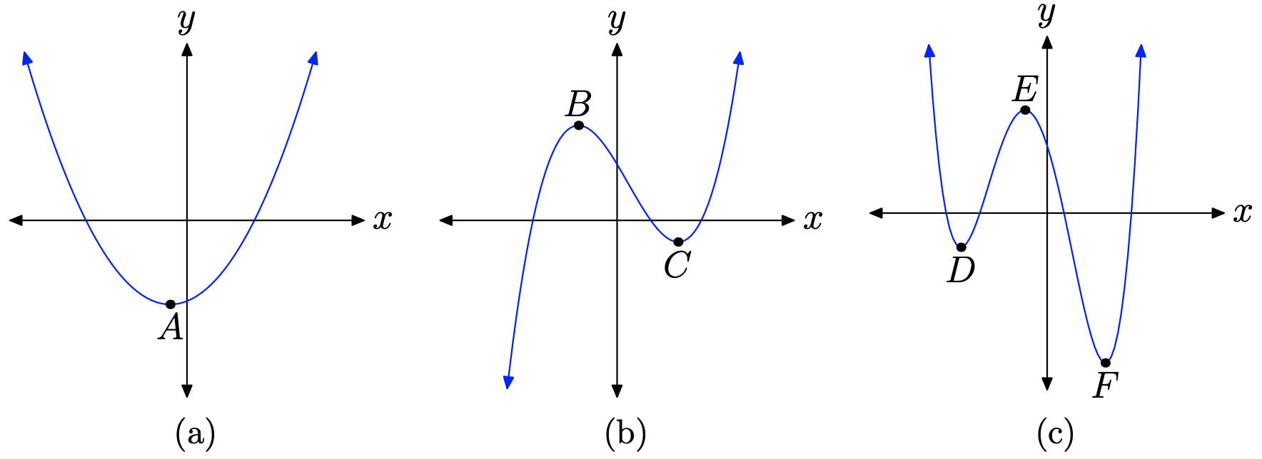
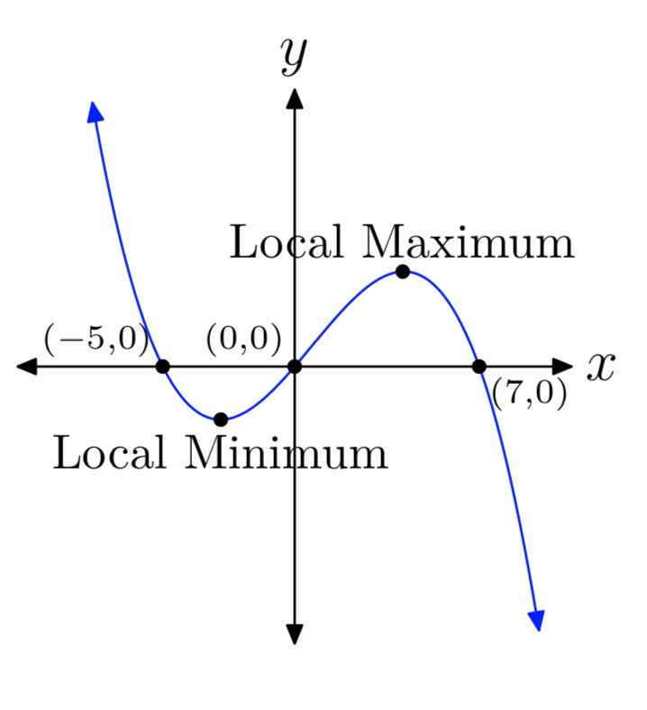
Finally, take a look at the graph in Figure \(\PageIndex{1c}\). Point F is the “absolute” lowest point on the graph, so the y-value of point F is an absolute minimum of the function. On the other hand, there is no highest point on the graph in Figure \(\PageIndex{1}\)(c), as each end of the graph escapes to positive infinity. Hence, the function has no absolute maximum.

Locally, point D in Figure \(\PageIndex{1}\)(c) is the lowest point, so the y-value of point D is a local minimum of the function. Similarly, in its immediate neighborhood, point E is the highest point, so the y-value of point E is a local maximum.

We now present the formal definitions.

Definition: Absolute Maximum

Suppose that \(c\) is in the domain of a function \(f\) and \(f(c) \geq f(x)\) for all \(x\) in the domain of \(f\). Then we say that \(f(c)\) is an absolute maximum of the function \(f\). Similarly, if \(f(c) \leq f(x)\) for all \(x\) in the domain of \(f\), then \(f(c)\) is an absolute minimum of the function \(f\).

The definition of local extrema is less restrictive.

Definition: Local Maximum

Let c be in the domain of \(f\). If \(f(c) \geq f(x)\) for all \(x\) in a neighborhood containing c, then we say that f(c) is a local maximum of the function f. On the other hand, if \(f(c) \leq f(x)\) for all \(x\) in a neighborhood containing \(c\), then we say that f(c) is a local minimum of the function f.

When mathematicians say “a neighborhood containing \(c\),” they usually mean a small open interval \((a, b)\) that contains \(c\).

Let’s explore the use of the graphing calculator in finding extrema.

Example \(\PageIndex{1}\)

Consider the polynomial function defined by the equation

\[p(x)=2(x-6)(x+2)(x+4). \nonumber \]

Use the graphing calculator to help find and classify all extrema of this function.

Solution

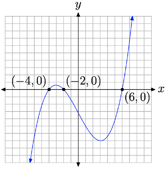
First, how much of the graph can you draw without the use of a calculator? The linear factors of \(p(x)\) are x − 6, x + 2, and x + 4, so the zeros are 6, −2, and −4, respectively. So we now know where the graph of p(x) crosses the x-axis.

To determine the end-behavior of \(p(x)\), we need to determine the leading term. It is not necessary to completely expand the polynomial with the distributive property.3 A little thought quickly reveals that if we were to do just that, the leading term in this case would be \(2x^{3}\). Consequently, as we sweep our eyes from left to right, the end-behavior of the polynomial should match that of its leading term \(2x^{3}\), rising from negative infinity, wiggling through its x-intercepts, then rising to positive infinity. The only choice is a graph similar to that in Figure \(\PageIndex{2}\).

Figure \(\PageIndex{2}\): The graph of \(p(x) = 2(x− 6)(x + 2)(x + 4)\) rises from negative infinity, wiggles through its x-intercepts, then continues to rise to positive infinity.

Note that the graph achieves a local maximum somewhere near x = −3 and a local minimum at approximately x = 3. We can find better approximations of the local extrema by using the maximum and minimum utilities in the CALC menu of the graphing calculator.

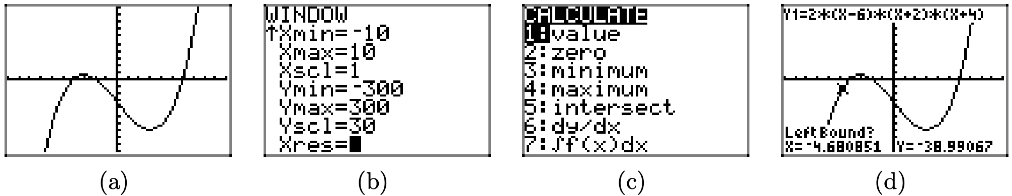
• First, plot the graph of the polynomial p(x) = 2(x − 6)(x + 2)(x + 4), as shown in Figure \(\PageIndex{3}\)(a), using the window parameters shown in Figure \(\PageIndex{3}\)(b).
• Open the CALCULATE menu by pressing 2nd CALC. This reveals a menu of choices as shown in Figure \(\PageIndex{3}\)(c). To start the utility to help find the local maximum near x = −3 (see Figure \(\PageIndex{2}\)), press 4:maximum on the menu.
• The utility responds by asking for a “Left Bound.” Use the arrow keys to move the cursor slightly left of the local maximum near x = −3, as shown in Figure \(\PageIndex{3}\)(d), then press the ENTER key.

Figure \(\PageIndex{3}\). Using the graphing calculator to determine the local maximum.

• The utility responds by asking for a “Right Bound.” Use the arrow keys to move the cursor slightly to the right of the local maximum near x = −3, as shown in Figure \(\PageIndex{4}\)(e), then press the ENTER key.
• The utility responds by asking for a “Guess.” Move the cursor so that it lies between the “Left Bound” and “Right Bound” made earlier, as shown in Figure \(\PageIndex{4}\)(f), then press the ENTER key. Anywhere between the left bound and right bound (note marks at top of screen in Figure \(\PageIndex{4}\)(f)) will do.

Figure \(\PageIndex{4}\). Using the graphing calculator to determine the local maximum (continued).

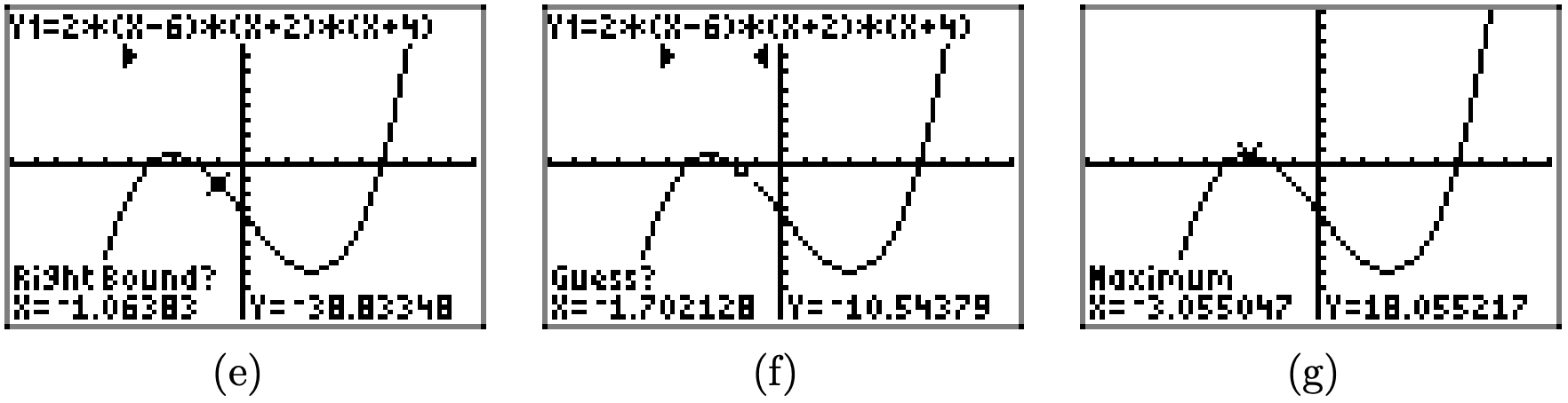
• The calculator responds by placing the cursor at the point where the local maximum occurs and reports its coordinates at the bottom of the screen, as shown in Figure \(\PageIndex{4}\)(g).

The coordinates of the point where the local maximum occurs are approximately \[(-3.055047,18.055217) \nonumber \]

We say that the function achieves a local maximum value of 18.055217 and that maximum occurs at \(x \approx-3.055047\).

In a similar manner, one can use the minimum utility in the CALC menu to find the local minimum that occurs near x = 3, as shown in Figure \(\PageIndex{5}\).

Figure \(\PageIndex{5}\). Use the minimum utility to find the local minimum.

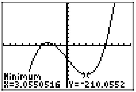
The coordinates of the point where the local minimum occurs are approximately \[(3.0550516,-210.0552) \nonumber \]

We say that the function achieves a local minimum value of −210.0552 and that minimum occurs at \(x \approx 3.0550516\).

Applications

In this section we will look at some applications that are modeled by polynomials.

Example \(\PageIndex{2}\)

A square piece of cardboard measures 24 inches per side. John cuts four smaller squares from each corner of the cardboard, tossing the material aside. He then bends up the sides of the remaining cardboard to form an open box with no top. Find the dimensions of the squares cut from each corner of the original piece of cardboard so that John maximizes the resulting volume of the box.

Solution

Let x represent the length of the side of the square cut from each corner of the larger square (see Figure \(\PageIndex{6}\)(a)). Because each side of the original square measures 24 inches, and we’re cutting two lengths of x inches off each end, the resulting length and width of the box is 24 − 2x inches (see Figure \(\PageIndex{6}\)(a) and/or (b)). When we toss away the square corners, then fold up the sides, we get a box with the dimensions shown in Figure \(\PageIndex{6}\)(b).

Figure \(\PageIndex{6}\): Material and resulting box.

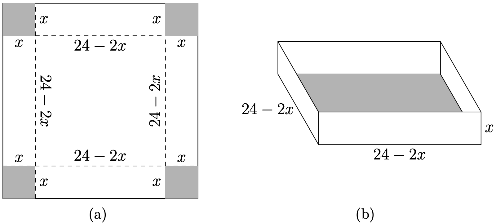
Because the volume of a box is computed by taking the product of the length and width of the base, multiplied by the height of the box, the volume of the box is given by the formula

\[V=x(24-2 x)(24-2 x) \nonumber \]

We can simplify equation (6) somewhat. Take a factor of 2 from each factor of 24−2x, as in

\[V=x(2)(12-x)(2)(12-x) \nonumber \]

then combine factors to write

\[V=4 x(12-x)^{2} \nonumber \]

We see that \(x\) and \(12 − x\) are linear factors of \(V\). Hence, the zeros of V are 0 and 12, respectively. Because 12−x is used as a factor twice, 2 is a “double root,” so the graph should be tangent to the x-axis at \(x = 2\).

If we were to expand Equation (7) completely, we would get a polynomial with leading term \(4x^{3}\). Hence, the end-behavior of our volume polynomial should match the end-behavior of its leading term, rising from negative infinity, wiggling through it zeros, then rising to positive infinity. However, because we have a “double root” at x = 2, we expect the graph to “kiss” the horizontal axis at this zero rather than pass through this zero.

Thus, the only possible shape the volume polynomial can assume is that shown in Figure \(\PageIndex{7}\).

Figure \(\PageIndex{7}\): The volume of the box as a function of the edge length of the removed squares.

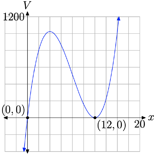
The domain of the polynomial defined by equation (7) is the set of all real numbers, or, in interval notation, \((-\infty, \infty)\). In Figure \(\PageIndex{7}\), if you project all the points on the graph onto the x-axis, the entire x-axis would be shaded, further indicating that the domain of the volume function is all real numbers.

However, this mathematical domain \((-\infty, \infty)\) ignores the fact that x represents the length of the square cut from each corner of the original square of cardboard (see Figure \(\PageIndex{6}\)(a)). You cannot cut a square having a side of negative length. Upon further inspection, the largest square that could be cut from each corner would have an edge measuring 12 inches. Remember, you have to cut four squares, one from each corner, and the edge of the original square piece of cardboard measures just 24 inches. Thus, the problem constrains x to the interval [0, 12]. This domain is called the empirical domain, or, if you will, the practical domain.

Definition: Empirical Domain

The empirical domain of a function is a subset of the mathematical domain, restricted so as to satisfy the constraints of the model.

Thus, only a portion of the graph in Figure \(\PageIndex{7}\) makes sense for this application— the part that is drawn over the empirical domain [0, 12], as shown in Figure \(\PageIndex{8}\).

Figure \(\PageIndex{8}\): Sketching the volume function over the empirical domain [0, 12].

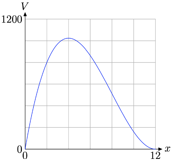
Remember, the original goal was to find the value of x that would maximize the volume of the box. A quick glance at the graph in Figure \(\PageIndex{8}\) shows that there is an absolute maximum (at least on the empirical domain [0, 12]) near x = 4. To obtain a better approximation, use the maximum utility in the CALC menu on your calculator, as we did to obtain the approximation shown in Figure \(\PageIndex{9}\)(b).

Figure \(\PageIndex{9}\). Finding the length of the edge that maximizes the volume of the box.

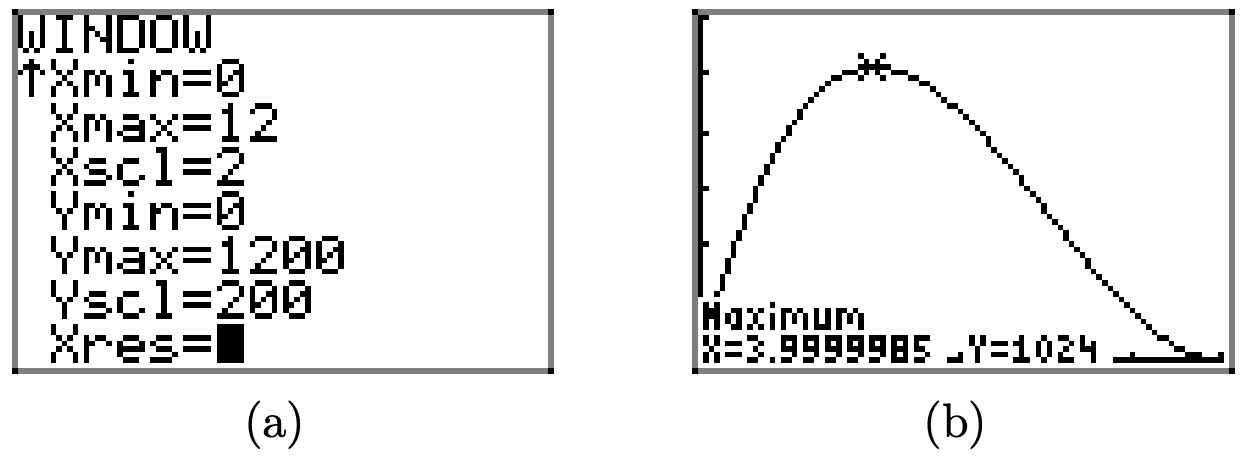
Indeed, it would appear that a maximum volume of 1024 cubic inches (\(V=1024 \mathrm{in}^{3}\)) is attained at \(x \approx 3.9999985\). It’s probably safe to say that the maximum volume occurs if squares having sides of length 4 inches are cut from the corners of the original piece of cardboard. The 3.9999985 probably contains a bit of error due to roundoff error on the calculator. Indeed, it is highly likely that some readers will get exactly x = 4 when they use the maximum utility, depending on the bounds and initial guess used, so don’t be worried if your calculator approximation differs slightly from ours.

Let’s look at another example.

Example \(\PageIndex{3}\)

Find the dimensions of the rectangle of largest area that has its base on the x-axis and its other two vertices above the x-axis and lying on the graph of the parabola \(y=4-x^{2}\).

Solution

The graph of \(y=4-x^{2}\) is a parabola that opens downward and is shifted upward 4 units. The right side of this equation factors

\[y=(2+x)(2-x) \nonumber \]

so the zeros of this function are −2 and 2. Because the rectangle has its base on the x-axis and its other vertices are on the parabola lying above the x-axis, we need only sketch the parabola on the domain [−2, 2] (see Figure \(\PageIndex{10}\)).

Figure \(\PageIndex{10}\): A rectangle inscribed under a parabola.

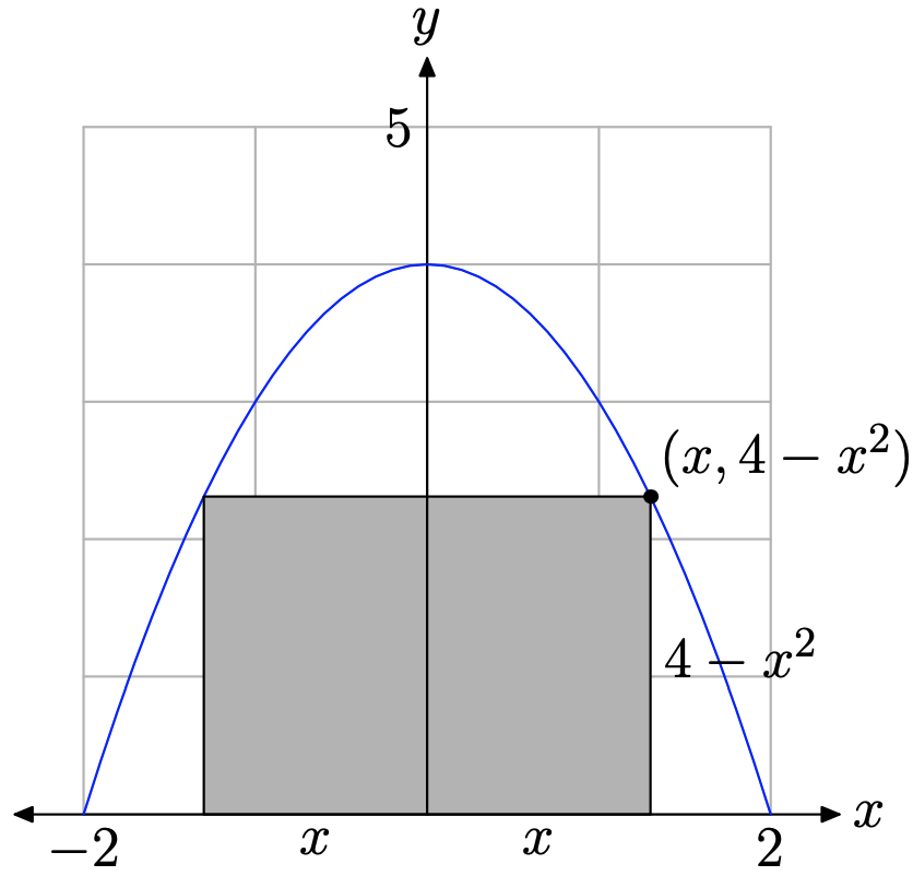
Because of symmetry, we can restrict x to the empirical domain [0, 2]. In Figure \(\PageIndex{10}\), note that we’ve selected a value of x from [0, 2], then plotted the point having this x-value on the parabola. Of course, the y-value of this point is \(y=4-x^{2}\). Thus, the height of the rectangle is \(4-x^{2}\) and the base (or width) of the rectangle is twice x, or 2x. The area of the rectangle is given by

\[A=\text { width } \cdot \text { height } \nonumber \]

Hence, the area A as a function of x is given by the polynomial

\[A=2 x\left(4-x^{2}\right) \nonumber \]

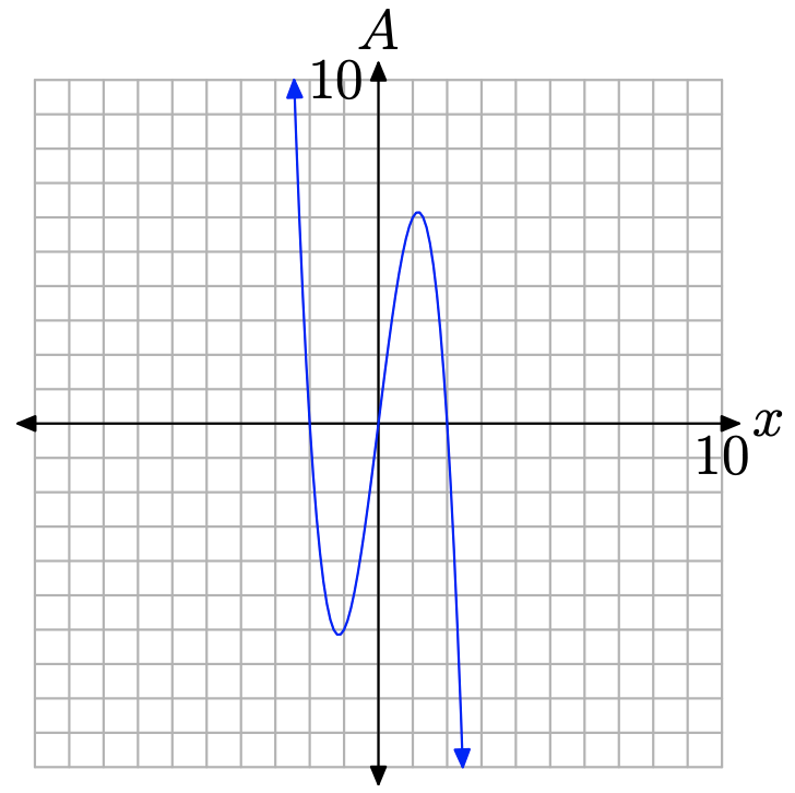
Note that equation (10) is a third degree polynomial having leading term \(-2 x^{3}\). Thus, the graph of the polynomial, as we sweep our eyes from left to right, must fall from positive infinity, wiggle through its x-intercepts, then continue falling to negative infinity.

We can factor equation (10) to obtain

\[A=2 x(2+x)(2-x) \nonumber \]

Therefore, the zeros of the polynomial are 0, −2, and 2, respectively. Thus, the polynomial must have shape similar to that shown in Figure \(\PageIndex{11}\). Note that the graph has x-intercepts at (−2, 0), (0, 0), and (2, 0).

Figure \(\PageIndex{11}\). The graph of the polynomial A = 2x(2 + x)(2 − x).

Because of the practical nature of this problem, we need to restrict x to the empirical domain [0, 2], as discussed above (see Figure \(\PageIndex{10}\). The graph of A = 2x(2 + x)(2 − x), restricted to the domain [0, 2], is shown in Figure \(\PageIndex{12}\).

Figure \(\PageIndex{12}\). The graph of the polynomial A = 2x(2 + x)(2 − x) restricted to the empirical domain [0, 2].

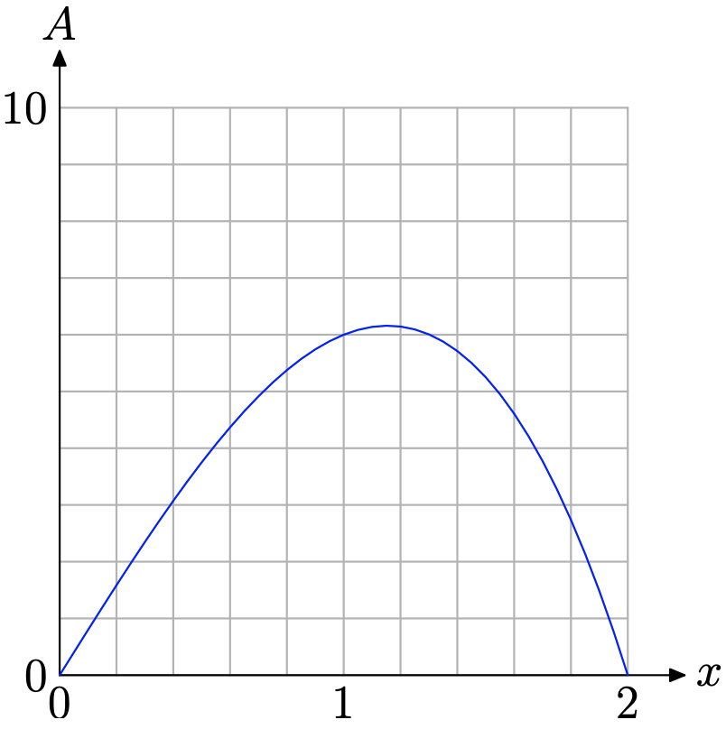
It appears (see Figure \(\PageIndex{12}\)) that A achieves an absolute maximum (at least on the empirical domain [0, 2]) near \(x \approx 1.2\). To obtain a better approximation, use the maximum utility in the CALC menu of the graphing calculator, as we did to obtain the approximation shown in Figure \(\PageIndex{13}\)(b).

Figure \(\PageIndex{13}\). Use the maximum utility to obtain an approximation of the maximum value of A.

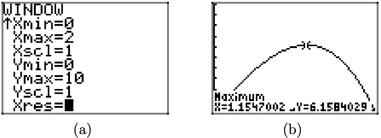
The result in Figure \(\PageIndex{13}\)(b) shows that we achieve a rectangle of maximum area \(A \approx 6.1584029\) if we choose \(x \approx 1.1547002\). Remember, your answers may differ slightly according to the left and right bounds you select, your guess, and also due to the inherent roundoff error in all calculators.

Exercise

In Exercises 1-8, perform each of the following tasks for the given polynomial.

1. Without the aid of a calculator, use an algebraic technique to identify the zeros of the given polynomial. Factor if necessary.
2. On graph paper, set up a coordinate system. Label each axis, but scale only the x-axis. Use the zeros and the end-behavior to draw a “rough graph” of the given polynomial with- out the aid of a calculator.
3. Classify each local extrema as a relative minimum or relative maximum.Note: It is not necessary to find the coordinates of the relative extrema. Indeed, this would be difficult with- out a calculator. All that is required is that you label each extrema as a relative maximum or minimum

Exercise \(\PageIndex{1}\)

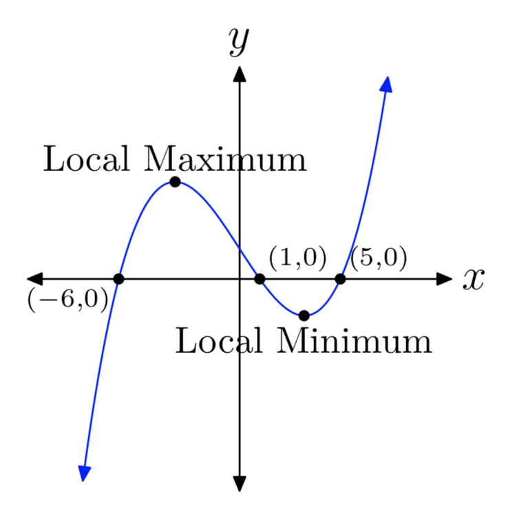
p(x) = (x+6)(x−1)(x−5)

Answer

Exercise \(\PageIndex{2}\)

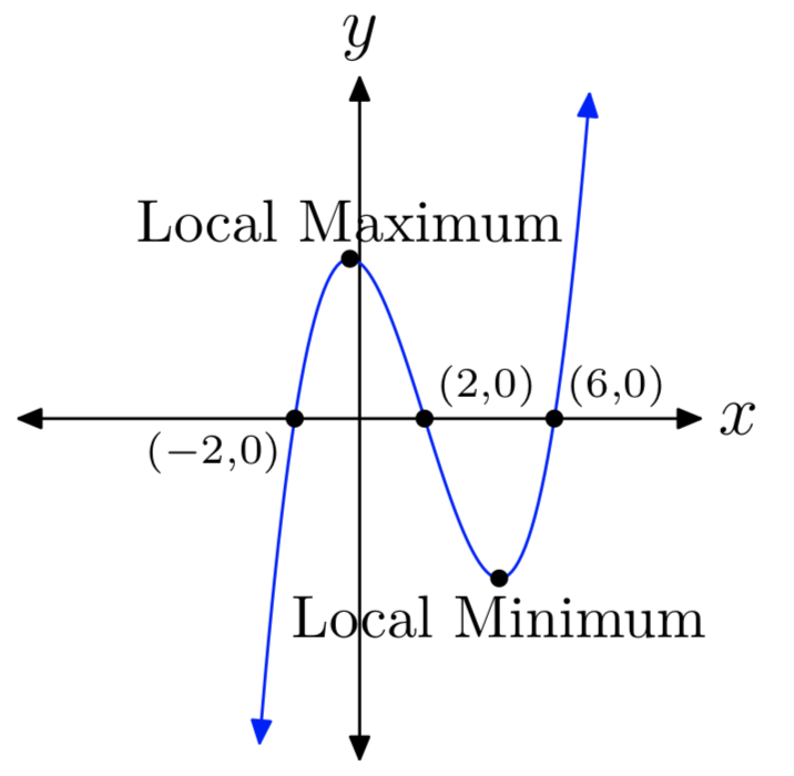
p(x) = (x+2)(x−4)(x−7)

Exercise \(\PageIndex{3}\)

\(p(x) = x^3−6x^2−4x+24\)

Answer

Exercise \(\PageIndex{4}\)

\(p(x) = x^3+x^2−36x−36\)

Exercise \(\PageIndex{5}\)

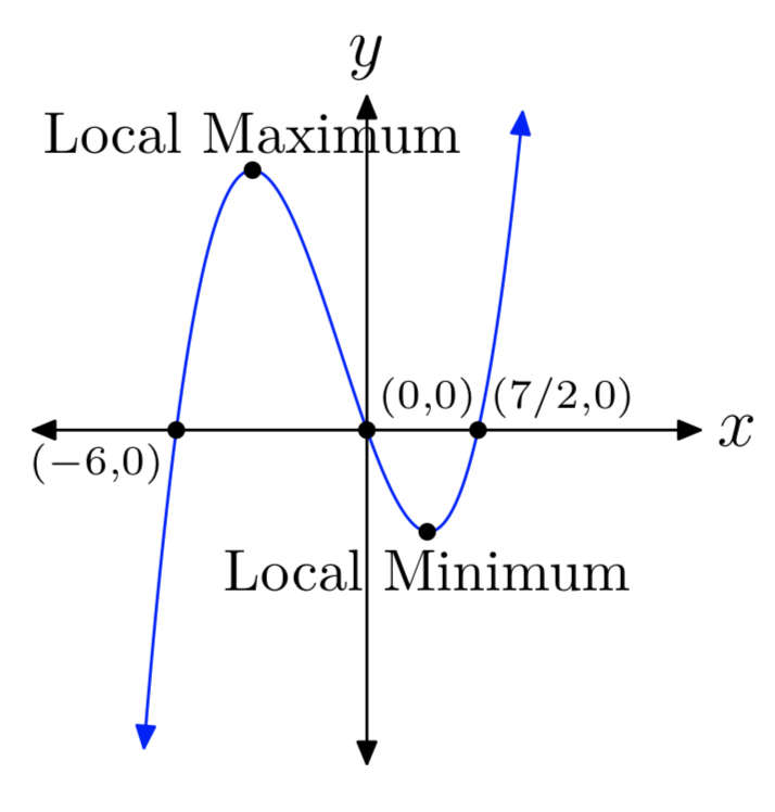
\(p(x) = 2x^3+5x^2−42x\)

Answer

Exercise \(\PageIndex{6}\)

\(p(x) = 2x^3−3x^2−44x\)

Exercise \(\PageIndex{7}\)

\(p(x) = −2x^3+4x^2+70x\)

Answer

Exercise \(\PageIndex{8}\)

\(p(x) = −6x^3−21x^2+90x\)

In Exercises 9-16, perform each of the following tasks for the given polynomial.

1. Use a graphing calculator to draw the graph of the polynomial. Adjust the viewing window so that the extrema or “turning points” of the polynomial are visible in the viewing window. Copy the resulting image onto your home- work paper. Label and scale each axis with xmin, xmax, ymin, and ymax.
2. Use the maximum and/or minimum utility in your calculator’s CALC menu to find the coordinates of the extrema. Label each extremum on your homework copy with its coordinates and state whether the extremum is a relative or absolute maximum or mini- mum.

Exercise \(\PageIndex{9}\)

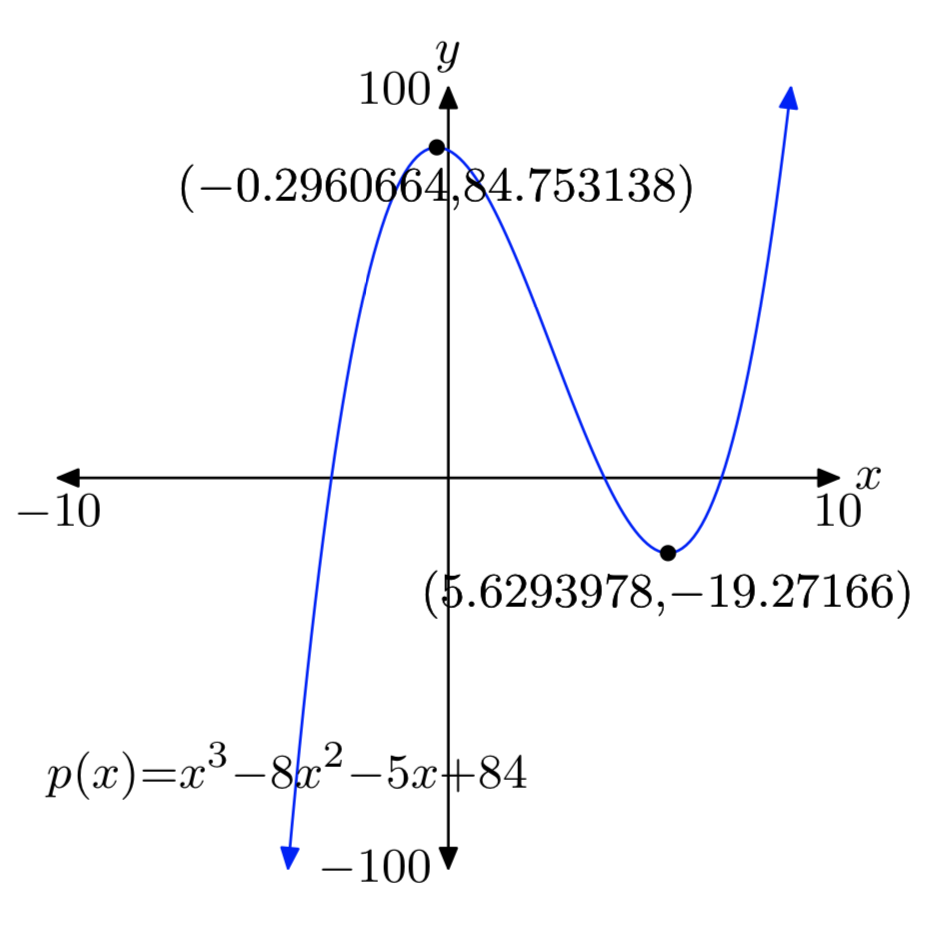
\(p(x) = x^3−8x^2−5x+84\)

Answer

Relative max: (−0.2960664, 84.753138)

Relative min: (5.6293978, −19.27166)

Answers may differ slightly due to round-off error.

Exercise \(\PageIndex{10}\)

\(p(x) = x^3+3x^2−33x−35\)

Exercise \(\PageIndex{11}\)

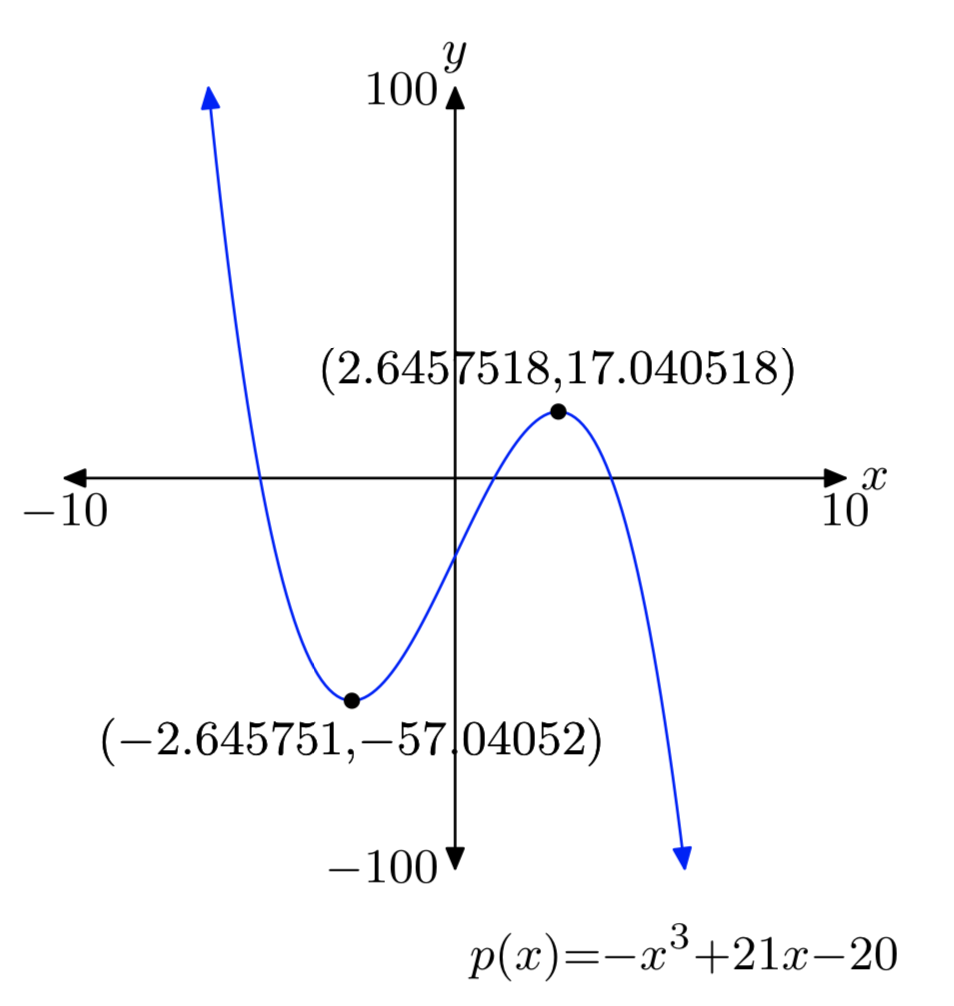
\(p(x) = −x^3+21x−20\)

Answer

Relative min: (−2.645751, −57.04052)

Relative max: (2.6457518, 17.040518)

Answers may differ slightly due to round-off error.

Exercise \(\PageIndex{12}\)

\(p(x) = −x^3+5x^2+12x−36\)

Exercise \(\PageIndex{13}\)

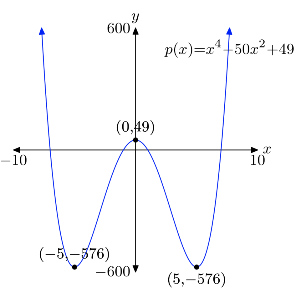
\(p(x) = x^4−50x^2+49\)

Answer

Absolute min: (−5, −576)

Relative max: (0, 49)

Absolute min: (5, −576)

Answers may differ slightly due to round-off error.

Exercise \(\PageIndex{14}\)

\(p(x) = x^4−29x^2+100\)

Exercise \(\PageIndex{15}\)

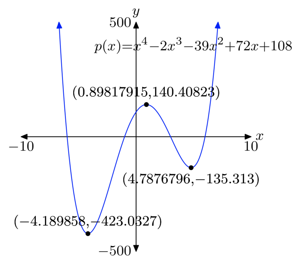
\(p(x) = x^4−2x^3−39x^2+72x+108\)

Answer

Absolute min: (−4.189858, −423.0327)

Relative max: (0.89817915, 140.40823)

Relative min: (4.7876796, −135.313)

Answers may differ slightly due to round-off error.

Exercise \(\PageIndex{16}\)

\(p(x) = x^4−3x^3−31x^2+63x+90\)

Exercise \(\PageIndex{17}\)

A square piece of cardboard measures 12 inches per side. Cherie cuts four smaller squares from each corner of the cardboard square, tossing the material aside. She then bends up the sides of the remaining cardboard to form an open box with no top. Find the dimensions of the squares cut from each corner of the original piece of cardboard so that Cherie maximizes the volume of the resulting box. Perform each of the following steps in your analysis.

1. Set up an equation that determines the volume of the box as a function of x, the length of the edge of each square cut from the four corners of the cardboard. Include any pictures used to determine this volume function.
2. State the empirical domain of the function created in part (a). Use your calculator to sketch the graph of the function over this empirical domain. Adjust the viewing window so that all extrema are visible in the viewing window.
3. Copy the image in your viewing window onto your homework paper. Label and scale each axis with xmin, xmax, ymin, and ymax. Use the maximum utility to find the coordinates of the absolute maximum on the function’s empirical domain.
4. What are the measures of the four squares cut from each corner of the original cardboard? What is the maximum volume of the box?

Answer

1. \(V = x(12−2x)^2\)
2. [0, 6]
3. Absolute max: (2, 128)
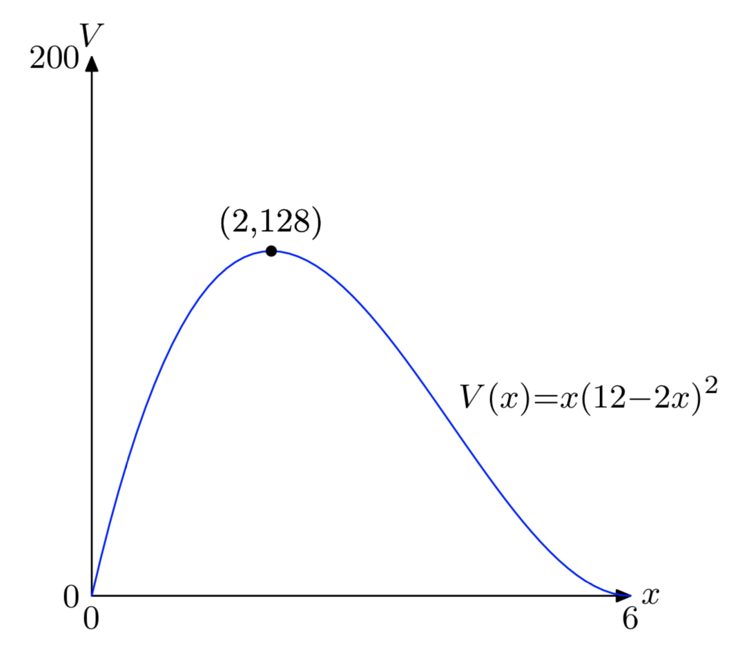
4. Cut square 2 inches on a side to produce a box having value 128 \(in^3\).

Exercise \(\PageIndex{18}\)

A rectangular piece of cardboard measures 8 inches by 12 inches. Schuyler cuts four smaller squares from each corner of the cardboard square, tossing the material aside. He then bends up the sides of the remaining cardboard to form an open box with no top. Find the dimensions of the squares cut from each corner of the original piece of cardboard so that Schuyler maximizes the volume of the resulting box. Perform each of the following steps in your analysis.

1. Set up an equation that determines the volume of the box as a function of x, the length of the edge of each square cut from the four corners of the cardboard. Include any pictures used to determine this volume function.
2. State the empirical domain of the function created in part (a). Use your calculator to sketch the graph of the function over this empirical domain. Adjust the viewing window so that all extrema are visible in the viewing window.
3. Copy the image in your viewing window onto your homework paper. Label and scale each axis with xmin, xmax, ymin, and ymax. Use the maximum utility to find the coordinates of the absolute maximum on the function’s empirical domain.
4. What are the measures of the four squares cut from each corner of the original cardboard? What is the maximum volume of the box?

Exercise \(\PageIndex{19}\)

Restrict the graph of the parabola \(y = 4−\frac{x^2}{4}\) to the first quadrant, then inscribe a rectangle inside the parabola, as shown in the figure that follows.

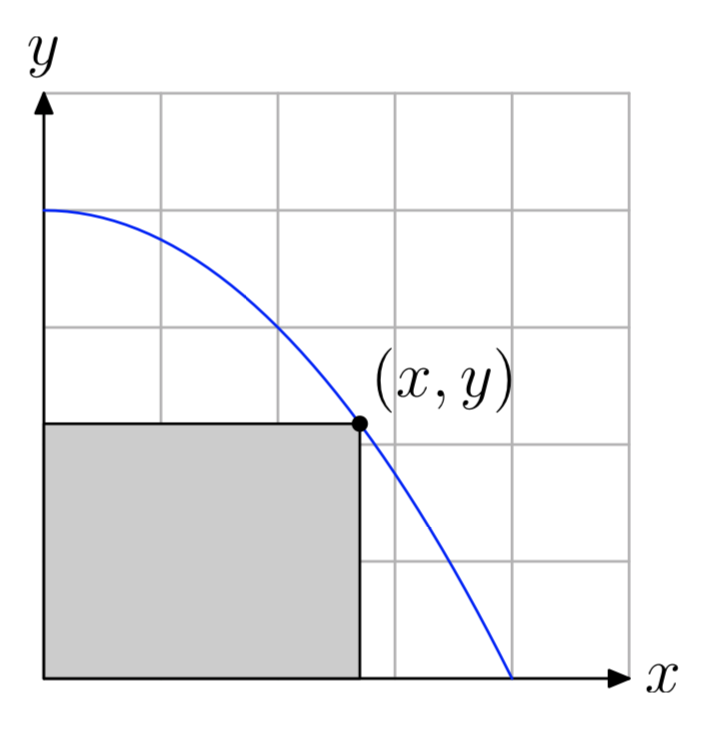
1. Express the area of the inscribed rectangle as a function of x.
2. State the empirical domain of the function defined in part (1). Use your calculator to graph the area function over its empirical domain. Adjust the window parameters so that all extrema are visible in the viewing window.
3. Copy the image in your viewing window to your homework paper. Label and scale each axis with xmin, xmax, ymin, and ymax. Use the maximum utility to find the coordinates of the absolute maximum on the function’s empirical domain. Label your graph with this result.
4. What are the dimensions of the rectangle of maximum area?

Answer

1. \(A = x(4−\frac{x^2}{4})\)
2. [0, 4]
3. Absolute max: (2.3094011, 6.1584029)
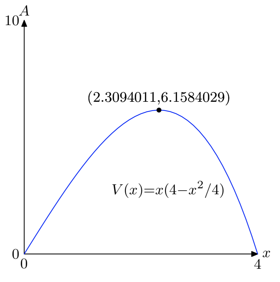
4. x = 2.3094011, y = 2.6666666

Exercise \(\PageIndex{20}\)

Restrict the graph of the parabola \(y = 4−\frac{x^2}{4}\) to the first quadrant, then inscribe a triangle inside the parabola, as shown in the figure that follows.

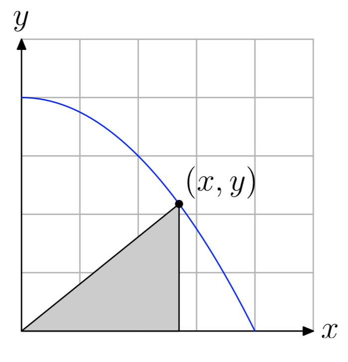
1. Express the area of the inscribed tri- angle as a function of x.
2. State the empirical domain of the function defined in part (a). Use your calculator to graph the area function over its empirical domain. Adjust the window parameters so that all extrema are visible in the viewing window.
3. Copy the image in your viewing window to your homework paper. Label and scale each axis with xmin, xmax, ymin, and ymax. Use the maximum utility to find the coordinates of the absolute maximum on the function’s empirical domain. Label your graph with this result.
4. What are the length of the base and height of the triangle of maximum area?

​​​​​​​