7.4: Point-Slope Form of a Line

Last updated
Save as PDF

Page ID: 31031

$ \newcommand{\vecs}[1]{\overset { \scriptstyle \rightharpoonup} {\mathbf{#1}} } $ $ \newcommand{\vecd}[1]{\overset{-\!-\!\rightharpoonup}{\vphantom{a}\smash {#1}}} $$\newcommand{\id}{\mathrm{id}}$ $ \newcommand{\Span}{\mathrm{span}}$ $ \newcommand{\kernel}{\mathrm{null}\,}$ $ \newcommand{\range}{\mathrm{range}\,}$ $ \newcommand{\RealPart}{\mathrm{Re}}$ $ \newcommand{\ImaginaryPart}{\mathrm{Im}}$ $ \newcommand{\Argument}{\mathrm{Arg}}$ $ \newcommand{\norm}[1]{\| #1 \|}$ $ \newcommand{\inner}[2]{\langle #1, #2 \rangle}$ $ \newcommand{\Span}{\mathrm{span}}$ $\newcommand{\id}{\mathrm{id}}$ $ \newcommand{\Span}{\mathrm{span}}$ $ \newcommand{\kernel}{\mathrm{null}\,}$ $ \newcommand{\range}{\mathrm{range}\,}$ $ \newcommand{\RealPart}{\mathrm{Re}}$ $ \newcommand{\ImaginaryPart}{\mathrm{Im}}$ $ \newcommand{\Argument}{\mathrm{Arg}}$ $ \newcommand{\norm}[1]{\| #1 \|}$ $ \newcommand{\inner}[2]{\langle #1, #2 \rangle}$ $ \newcommand{\Span}{\mathrm{span}}$$\newcommand{\AA}{\unicode[.8,0]{x212B}}$

In the previous section we learned that if we are provided with the slope of a line and its $y$-intercept, then the equation of the line is $y = mx + b$, where $m$ is the slope of the line and $b$ is the $y$-coordinate of the line’s $y$-intercept.

However, suppose that the $y$-intercept is unknown? Instead, suppose that we are given a point $(x_0,y_0)$ on the line and we’re also told that the slope of the line is m (see Figure $\PageIndex{1}$).

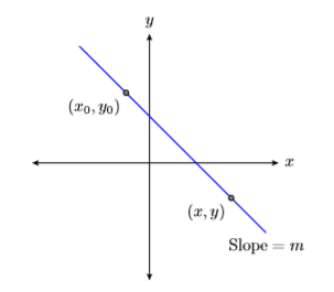
fig 3.5.1.png — Figure $\PageIndex{1}$: A line through the point $(x_0,y_0)$ with slope $m$.

Let $(x,y)$ be an arbitrary point on the line, then use the points $(x_0,y_0)$ and $(x,y)$ to calculate the slope of the line.

\[\begin{aligned} \text { Slope }&= \dfrac{\Delta y}{\Delta x} \quad \color{Red} \text { The slope formula. } \\ m&= \dfrac{y-y_{0}}{x-x_{0}} \quad \color{Red} \text { Substitute } m \text { for the slope. Use }(x, y) \text { and }\left(x_{0}, y_{0}\right) \text { to calculate the difference in } y \text { and the difference in } x \end{aligned} \nonumber \]

Clear the fractions from the equation by multiplying both sides by the common denominator.

\[\begin{aligned} m\left(x-x_{0}\right)&= \left[\dfrac{y-y_{0}}{x-x_{0}}\right]x-x_{0} \quad \color{Red} \text { Multiply both sides by } x-x_{0} \\ m\left(x-x_{0}\right)&= y-y_{0} \qquad \qquad \color{Red} \text { Cancel. } \end{aligned} \nonumber \]

Thus, the equation of the line is $y−y_0 = m(x−x-0)$.

The Point-Slope form of a line

The equation of the line with slope m that passes through the point $\left(x_{0}, y_{0}\right)$ is: \[y-y_{0}=m\left(x-x_{0}\right) \nonumber \]

Example $\PageIndex{1}$

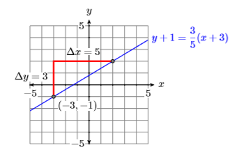
Draw the line passing through the point $(−3,−1)$ that has slope $3/5$, then label it with its equation.

Solution

Plot the point $(−3,−1)$, then move $3$ units up and $5$ units to the right (see Figure $\PageIndex{2}$). To ﬁnd the equation, substitute $(−3,−1)$ for $(x_0,y_0)$ and $3/5$ for m in the point-slope form of the line.

\[\begin{aligned} {y-y_{0}} &= m\left(x-x_{0}\right) \quad \color{Red} \text { Point-slope form. } \\ y-(-1) &= \dfrac{3}{5}(x-(-3)) \quad \color{Red} \text { Substitute: } 3 / 5 \text { for } m,-3 \text { for } x_{0}, \text { and }-1 \text { for } y_{0} \end{aligned} \nonumber \]

Simplifying, the equation of the line is $y+1=\dfrac{3}{5}(x+3)$.

fig 3.5.2.png — Figure $\PageIndex{2}$: The line passing through $(−3,−1)$ with slope $3/5$.

Exercise $\PageIndex{1}$

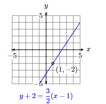
Draw the line passing through the point $(1,−2)$ that has slope $3/2$, then label it with its equation.

Answer: $Exercise 3.5.1.png$

At this point, you may be asking the question “When should I use the slopintercept form and when should I use the point-slope form?” Here is a good tip.

Tip: Which form should I use

The form you should select depends upon the information given.

If you are given the $y$-intercept and the slope, use $y = mx + b$.
If you are given a point and the slope, use $y−y_0 = m(x−x_0)$.

Example $\PageIndex{2}$

Find the equation of the line passing through the points $P(−1,2)$ and $Q(3,−4)$.

Solution

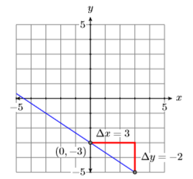
First, plot the points $P(−1,2)$ and $Q(3,−4)$ and draw a line through them (see Figure $\PageIndex{3}$).

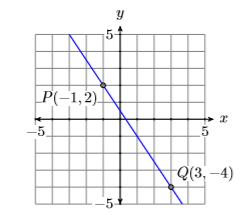
fig 3.5.3.png — Figure $\PageIndex{3}$: The line passing through $P(−1,2)$ and $Q(3,−4)$.

Next, let’s calculate the slope of the line by subtracting the coordinates of the point $P(−1,2)$ from the coordinates of point $Q(3,−4)$.

\[\begin{aligned} \text { Slope } &=\dfrac{\Delta y}{\Delta x} \\ &=\dfrac{-4-2}{3-(-1)} \\ &=\dfrac{-6}{4} \\ &=-\dfrac{3}{2} \end{aligned} \nonumber \]

Thus, the slope is $−3/2$.

Next, use the point-slope form $y−y_0 = m(x−x_0)$ to determine the equation of the line. It’s clear that we should substitute $−3/2$ form. But which of the two points should we use? If we use the point $P(−1,2)$ for $(x_0,y_0)$, we get the answer on the left, but if we use the point $Q(3,−4)$ for $(x_0,y_0)$, we get the answer on the right.

$y-2=-\dfrac{3}{2}(x-(-1)) \qquad$ or $\qquad y-(-4)=-\dfrac{3}{2}(x-3)$

At ﬁrst glance, these answers do not look the same, but let’s examine them a bit more closely, solving for $y$ to put each in slope-intercept form. Let’s start with the equation on the left.

\[\begin{aligned}
y-2 &= -\dfrac{3}{2}(x-(-1)) \quad \color{Red} \text { Using } m=-3 / 2 \text { and }\left(x_{0}, y_{0}\right)=(-1,2) \\
y-2 &= -\dfrac{3}{2}(x+1) \quad \color{Red} \text { Simplify. } \\
y-2 &= -\dfrac{3}{2} x-\dfrac{3}{2} \quad \color{Red} \text { Distribute }-3 / 2\\
y-2+2 &= -\dfrac{3}{2} x-\dfrac{3}{2}+2 \quad \color{Red} \text { Add } 2 \text { to both sides. } \\
y &= -\dfrac{3}{2} x-\dfrac{3}{2}+\dfrac{4}{2} \quad \color{Red} \text { On the left, simplify. On the right, make equivalent fractions with a common denominator. } \\
y &= -\dfrac{3}{2} x+\dfrac{1}{2} \quad \color{Red} \text { Simplify. }
\end{aligned} \nonumber \]

Let’s put the second equation in slope-intercept form.

Note

Note that the form $y=-\dfrac{3}{2} x+\dfrac{1}{2}$, when compared with the general slope-intercept form $y = mx + b$, indicates that the $y$-intercept is $(0,1/2)$. Examine Figure $\PageIndex{3}$. Does it appear that the $y$-intercept is $(0,1/2)$?

\[\begin{aligned}
y-(-4) &= -\dfrac{3}{2}(x-3) \quad \color{Red} \text { Using } m=-3 / 2 \text { and }\left(x_{0}, y_{0}\right)=(3,-4) \\
y+4 &= -\dfrac{3}{2}(x-3) \quad \color{Red} \text { Simplify. } \\
y+4 &= -\dfrac{3}{2} x+\dfrac{9}{2} \quad \color{Red}\text { Distribute }-3 / 2\\
y+4-4 &= -\dfrac{3}{2} x+\dfrac{9}{2}-4 \quad \color{Red} \text { Subtract } 4 \text { from both sides. } \\
y &= -\dfrac{3}{2} x + \dfrac{9}{2}-\dfrac{8}{2} \quad \color{Red} \text { On the left, simplify. On the right, make equivalent fractions with a common denominator. }\\
y &= -\dfrac{3}{2} x+\dfrac{1}{2}
\end{aligned} \nonumber \]

Thus, both equations simplify to the same answer, $y=-\dfrac{3}{2} x+\dfrac{1}{2}$. This means that the equations $y-2=-\dfrac{3}{2}(x-(-1))$ and $y-(-4)=-\dfrac{3}{2}(x-3)$, though they look diﬀerent, are the same.

Exercise $\PageIndex{2}$

Find the equation of the line passing through the points $P(−2,1)$ and $Q(4,−1)$.

Answer: $y=-\dfrac{1}{3} x+\dfrac{1}{3}$

Example $\PageIndex{2}$ gives rise to the following tip.

tip

When ﬁnding the equation of a line through two points $P$ and $Q$, you may substitute either point $P$ or $Q$ for $(x_0,y_0)$ in the point-slope form $y−y_0 = m(x−x_0)$. The results look diﬀerent, but they are both equations of the same line.

Parallel Lines

Recall that slope is a number that measures the steepness of the line. If two lines are parallel (never intersect), they have the same steepness.

Parallel lines

If two lines are parallel, they have the same slope.

Example $\PageIndex{3}$

Sketch the line $y=\dfrac{3}{4} x-2$, then sketch the line passing through the point $(−1,1)$ that is parallel to the line $y=\dfrac{3}{4} x-2$. Find the equation of this parallel line.

Solution

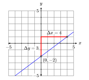
Note that $y=\dfrac{3}{4} x-2$ is in slope-intercept form $y = mx+b$. Hence,its slope is $3/4$ and its $y$-intercept is $(0,−2)$. Plot the $y$-intercept $(0,−2)$, move up $3$ units, right $4$ units, then draw the line (see Figure $\PageIndex{4}$).

fig 3.5.4.png — Figure $\PageIndex{4}$: The line $y=\dfrac{3}{4} x-2$.

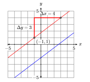
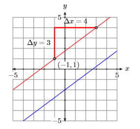
The second line must be parallel to the ﬁrst, so it must have the same slope $3/4$. Plot the point $(−1,1)$, move up $3$ units, right $4$ units, then draw the line (see the red line in Figure $\PageIndex{5}$).

fig 3.5.5.png — Figure $\PageIndex{5}$: Adding a line parallel to $y=\dfrac{3}{4} x-2$.

To ﬁnd the equation of the parallel red line in Figure $\PageIndex{5}$, use the point slope form, substitute $3/4$ for $m$, then $(−1,1)$ for $(x_0,y_0)$. That is, substitute $−1$ for $x_0$ and $1$ for $y_0$.

\[\begin{aligned} y-y_{0}&= m\left(x-x_{0}\right) \quad \color{Red} \text { Point-slope form. } \\ y-1&= \dfrac{3}{4}(x-(-1)) \quad \color{Red} \text { Substitute: } 3 / 4 \text { for } m,-1 \text { for } x_{0} \text { and } 1 \text { for } y_{0} \\ y-1&= \dfrac{3}{4}(x+1) \quad \color{Red} \text { Simplify. } \end{aligned} \nonumber \]

Check: In this example, we were not required to solve for $y$, so we can save ourselves some checking work by writing the equation

$y-1=\dfrac{3}{4}(x+1) \qquad$ in the form $\qquad y=\dfrac{3}{4}(x+1)+1$

by adding $1$ to both sides of the ﬁrst equation.

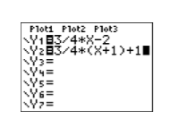
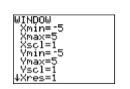
Next, enter each equation as shown in Figure $\PageIndex{6}$, then change the WINDOW setting as shown in Figure $\PageIndex{7}$.

fig 3.5.6.png — Figure $\PageIndex{6}$: Enter equations of parallel lines.

fig 3.5.7.png — Figure $\PageIndex{7}$: Adjust the **WINDOW** parameters as shown.

Next, press the GRAPH button, the select 5:ZSquare to produce the image in Figure $\PageIndex{9}$.

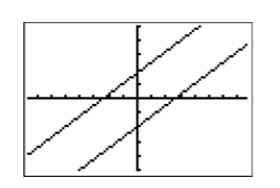
fig 3.5.8.png — Figure $\PageIndex{8}$: Hand-drawn parallel lines.

fig 3.5.9.png — Figure $\PageIndex{9}$: Press the GRAPH button then select **5:ZSquare** to produce this image.

Note the close correlation of the calculator lines in Figure $\PageIndex{9}$ to the hand drawn lines in Figure $\PageIndex{8}$. This gives us conﬁdence that we’ve captured the correct answer.

Exercise $\PageIndex{3}$

Find the equation of the line which passes through the point $(2,−3)$ and is parallel to the line $y=\dfrac{3}{4} x+2$.

Answer: $y=\dfrac{3}{2} x-6$

Perpendicular Lines

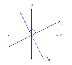
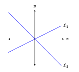
Two lines are perpendicular if they meet and form a right angle ($90$ degrees). For example, the lines $\mathcal{L}_{1}$ and $\mathcal{L}_{2}$ in Figure $\PageIndex{10}$ are perpendicular, but the lines $\mathcal{L}_{1}$ and $\mathcal{L}_{2}$ in Figure $\PageIndex{11}$ are not perpendicular.

fig 3.5.10.png — Figure $\PageIndex{10}$: The lines $\mathcal{L}_{1}$ and $\mathcal{L}_{2}$ are perpendicular. They meet and form a right angle ($90$ degrees).

fig 3.5.11.png — Figure $\PageIndex{11}$: The lines $\mathcal{L}_{1}$ and $\mathcal{L}_{2}$ are **not** perpendicular. They do **not** form a right angle ($90$ degrees).

Before continuing, we need to establish a relation between the slopes of two perpendicular lines. So, consider the perpendicular lines $\mathcal{L}_{1}$ and $\mathcal{L}_{2}$ in Figure $\PageIndex{12}$.

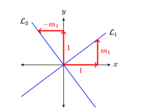
fig 3.5.12.png — Figure $\PageIndex{12}$: Perpendicular lines $\mathcal{L}_{1}$ and $\mathcal{L}_{2}$.

Note

If we were to rotate line $\mathcal{L}_{1}$ ninety degrees counter-clockwise, then $\mathcal{L}_{1}$ would align with the line $\mathcal{L}_{2}$, as would the right triangles revealing their slopes.
$\mathcal{L}_{1}$ has slope $\dfrac{\Delta y}{\Delta x}=\dfrac{m_{1}}{1}=m_{1}$.
$\mathcal{L}_{2}$ has slope $\dfrac{\Delta y}{\Delta x}=\dfrac{1}{-m_{1}}=-\dfrac{1}{m_{1}}$

Slopes of perpendicular lines

If $\mathcal{L}_{1}$ and $\mathcal{L}_{2}$ are perpendicular lines and $\mathcal{L}_{1}$ has slope $m_1$, the $\mathcal{L}_{2}$ has slope $−1/m_1$. That is, the slope of $\mathcal{L}_{2}$ is the negative reciprocal of the slope of $\mathcal{L}_{1}$.

Examples:

To ﬁnd the slope of a perpendicular line, invert the slope of the ﬁrst line and negate.

If the slope of $\mathcal{L}_{1}$ is $2$, then the slope of the perpendicular line $\mathcal{L}_{2}$ is $−1/2$.
If the slope of $\mathcal{L}_{1}$ is $−3/4$, then the slope of the perpendicular line $\mathcal{L}_{2}$ is $4/3$.

Example $\PageIndex{4}$

Sketch the line $y=-\dfrac{2}{3} x-3$, then sketch the line through $(2,1)$ that is perpendicular to the line $y=-\dfrac{2}{3} x-3$. Find the equation of this perpendicular line.

Solution

Note that $y=-\dfrac{2}{3} x-3$ is in slope-intercept form $y = mx+b$. Hence, its slope is $−2/3$ and its $y$-intercept is $(0,−3)$. Plot the $y$-intercept $(0,−3)$, move right $3$ units, down two units, then draw the line (see Figure $\PageIndex{13}$).

fig 3.5.13.png — Figure $\PageIndex{13}$: The line $y=-\dfrac{2}{3} x-3$.

Because the line $y=-\dfrac{2}{3} x-3$ has slope $−2/3$, the slope of the line perpendicular to this line will be the negative reciprocal of $−2/3$, namely $3/2$. Thus, to draw the perpendicular line, start at the given point $(2 ,1)$, move up $3$ units, right $2$ units, then draw the line (see Figure $\PageIndex{14}$).

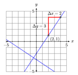
fig 3.5.14.png — Figure $\PageIndex{14}$: Adding a line perpendicular to $y=-\dfrac{2}{3} x-3$.

To ﬁnd the equation of the perpendicular line in Figure $\PageIndex{14}$, use the point slope form, substitute $3/2$ for $m$, then $(2 ,1)$ for $(x_0,y_0)$. That is, substitute $2$ for $x_0$, then $1$ for $y_0$.

\[\begin{aligned} y-y_{0}&= m\left(x-x_{0}\right) \quad \color{Red} \text { Point-slope form. } \\ y-1&= \dfrac{3}{2}(x-2) \quad \color{Red} \text { Substitute: } 3 / 2 \text { for } m, 2 \text { for } x_{0} \text { and } 1 \text { for } y_{0} \end{aligned} \nonumber \]

Check: In this example, we were not required to solve for $y$, so we can save ourselves some checking work by writing the equation

$y-1=\dfrac{3}{2}(x-2) \qquad$ in the form $\quad y=\dfrac{3}{2}(x-2)+1$

by adding $1$ to both sides of the ﬁrst equation. Next, enter each equation as shown in Figure $\PageIndex{15}$, then select 6:ZStandard to produce the image in Figure $\PageIndex{16}$.

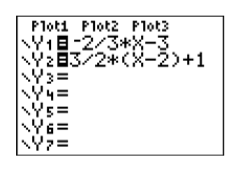
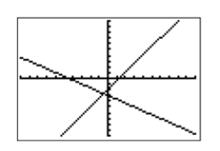
fig 3.5.15.png — Figure $\PageIndex{15}$: Enter equations of perpendicular lines.

fig 3.5.16.png — Figure $\PageIndex{16}$: **6:ZStandard** produces two lines that do not look perpendicular.

Note that the lines in Figure $\PageIndex{16}$ do not appear to be perpendicular. Have we done something wrong? The answer is no! The fact that the calculator’s viewing screen is wider than it is tall is distorting the angle at which the lines meet.

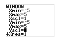
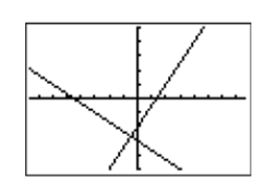
To make the calculator result match the result in Figure $\PageIndex{14}$, change the window settings as shown in Figure $\PageIndex{17}$, then select 5:ZSquare from the ZOOM menu to produce the image in Figure $\PageIndex{18}$. Note the close correlation of the calculator lines in Figure $\PageIndex{18}$ to the hand-drawn lines in Figure $\PageIndex{14}$. This gives us conﬁdence that we’ve captured the correct answer.

fig 3.5.17.png — Figure $\PageIndex{17}$: Change the **WINDOW** parameters as shown.

fig 3.5.18.png — Figure $\PageIndex{18}$: **5:ZSquare** produces two lines that do look perpendicular.

Exercise $\PageIndex{4}$

Find the equation of the line that passes through the point $(−3,1)$ and is perpendicular to the line $y=-\dfrac{1}{2} x+1$.

Answer: $y=2 x+7$

Applications

Let’s look at a real-world application of lines.

Example $\PageIndex{5}$

Water freezes at $32^{\circ} \mathrm{F}$ (Fahrenheit) and at $0^{\circ} \mathrm{C}$ (Celsius). Water boils at $212^{\circ} \mathrm{F}$ and at $100^{\circ} \mathrm{C}$. If the relationship is linear, ﬁnd an equation that expresses the Celsius temperature in terms of the Fahrenheit temperature. Use the result to ﬁnd the Celsius temperature when the Fahrenheit temperature is $113^{\circ} \mathrm{F}$.

Solution

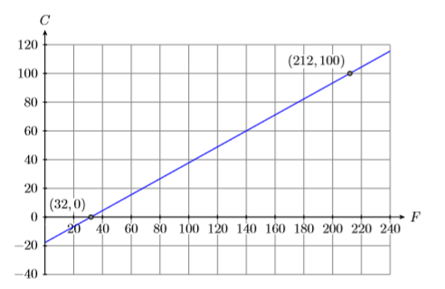
In this example, the Celsius temperature depends on the Fahrenheit temperature. This makes the Celsius temperature the dependent variable and it gets placed on the vertical axis. This Fahrenheit temperature is the independent variable, so it gets placed on the horizontal axis (see Figure $\PageIndex{19}$).

Next, water freezes at $32^{\circ} \mathrm{F}$ and $0^{\circ} \mathrm{C}$, giving us the point $(F,C) = (32,0)$. Secondly, water boils at $212^{\circ} \mathrm{F}$ and $100^{\circ} \mathrm{C}$, giving us the point $(F,C)= (212,100)$. Note how we’ve scaled the axes so that each of these points ﬁt on the coordinate system. Finally, assuming a linear relationship between the Celsius and Fahrenheit temperatures, draw a line through these two points (see Figure $\PageIndex{19}$).

fig 3.5.19.png — Figure $\PageIndex{19}$: The linear relationship between Celsius and Fahrenheit temperature.

Calculate the slope of the line.

\[\begin{aligned} m&= \dfrac{\Delta C}{\Delta F} \quad \color{Red} \text { Slope formula. } \\ m&= \dfrac{100-0}{212-32} \quad \color{Red} \text { Use the points }(32,0) \text { and }(212,100) \text { to compute the difference in C and F}\\ m&= \dfrac{100}{180} \quad \color{Red} \text { Simplify. } \\ m&= \dfrac{5}{9} \quad \color{Red} \text { Reduce. } \end{aligned} \nonumber \]

You may either use $(32,0)$ or $(212,100)$ in the point-slope form. The point $(32,0)$ has smaller numbers, so it seems easier to substitute $(x_0,y_0) = (32 ,0)$ and $m =5 /9$ into the point-slope form $y−y_0 = m(x−x_0)$.

\[\begin{aligned} y-y_{0}=& m\left(x-x_{0}\right) \quad \color{Red} \text { Point-slope form. } \\ y-0 &=\dfrac{5}{9}(x-32) \quad \color{Red} \text { Substitute: } 5 / 9 \text { for } m, 32 \text { for } x_{0}, \text { and } 0 \text { for } y_{0} \\ y &=\dfrac{5}{9}(x-32) \quad \color{Red} \text { Simplify. } \end{aligned} \nonumber \]

However, our vertical and horizontal axes are labeled $C$ and $F$ (see Figure $\PageIndex{19}$) respectively, so we must replace $y$ with $C$ and $x$ with $F$ to obtain an equation expressing the Celsius temperature $C$ in terms of the Fahrenheit temperature $F$.

\[C=\dfrac{5}{9}(F-32) \label{temperature} \]

Finally, to ﬁnd the Celsius temperature when the Fahrenheit temperature is $113^{\circ} \mathrm{F}$, substitute $113$ for $F$ in Equation \ref{temperature}

\[\begin{aligned} C&= \dfrac{5}{9}(F-32) \quad \color{Red} \text { Equation }(3.5.1) \\ C&= \dfrac{5}{9}(113-32) \quad \color{Red} \text { Substitute: } 113 \text { for } F \\ C&= \dfrac{5}{9}(81) \quad \color{Red} \text { Subtract. } \\ C&= 45 \quad \color{Red} \text { Multiply. } \end{aligned} \nonumber \]

Therefore, if the Fahrenheit temperature is $113^{\circ} \mathrm{F}$, then the Celsius temperature is $45^{\circ} \mathrm{C}$.

Exercise $\PageIndex{5}$

Find an equation that expresses the Fahrenheit temperature in terms of the Celsius temperature. Use the result to ﬁnd the Fahrenheit temperature when the Celsius temperature is $25^{\circ} \mathrm{C}$.

Answer: $77^{\circ} \mathrm{F}$