1.6: Exponents and Radicals

Learning Objectives

By the end of this section, you will be able to:

• Simplify expressions with roots
• Estimate and approximate roots
• Simplify variable expressions with roots

Warm Up

Compute the following:

1. \(4\cdot 4\)
2. \(9 \cdot 9\)
3. \(64 \div 8\)
4. \(9\div 3\)

Answer

1. 16
2. 81
3. 8
4. 3

Exponents

Exponents are notation we use to multiply a number to itself multiple times. We take the number we want to multiply by as the big number and how many times we want to multiply by it as the smaller one on top. For example, take \(4\cdot 4\) we can write this as \(4^2\) read as "4 to the 2".

How about \(4\cdot 4\cdot 4\cdot 4\cdot 4\cdot 4\)? Here we have 4 multiplied to itself 5 times, so we can express this as \(4^5\) read "4 to the 5".

We can see that if we have \(4^2\cdot 4\) then this would be \(4^3\) since \(4^2=4\cdot 4\) and that \(4^2\cdot 4=4\cdot 4\cdot 4=4^3\) as we have 4 multiplied to itself 3 times. (By the way \(4^3=64\)

We can go back as well if we take \(4^3\div 4\) then this would be \(4^2\) since \(4^3=4\cdot 4\cdot 4\) and that \(4^3\div 4=4\cdot 4\cdot 4\div 4=4^2\) as we have 4 multiplied to itself 2 times. (By the way \(4^2=16\))

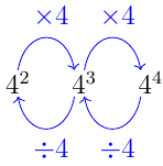
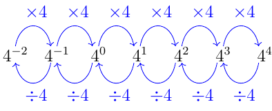
We see that multiplying by 4 we go up an exponent and down an exponent by dividing by 4.

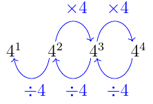
What if we divide \(4^2\) by 4, what would we get? We would get \(4^2\div 4=4\cdot 4\div 4=4=4^1\). Which make sense because we have only one 4.

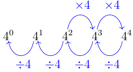
What if we do it again? What if we divide by 4 again to get \(4^0\)? What is \(4^0\)? Well \(4^1\div 4=4\div 4=1=4^0\).

Do it again. What is \(4^{-1}\)? \(4^0\div 4=1\div 4=\frac{1}{4}=4^{-1}\)

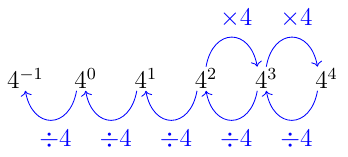
And again. What is \(4^{-2}\)? \(4^{-1}\div 4=1\div {4\cdot 4}=\frac{1}{16}=\frac{1}{4^2}=4^{-2}\)

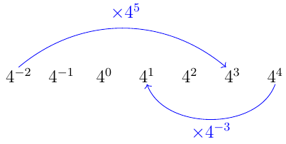
Instead of counting multiplying by 4 everytime, we can "jump" by multiplying by multiple copies of 4. For example, if we wanted to get from \(4^{-2}\) to \(4^3\) we would multiple by \(4^5\). Why? We notice that the difference between 3 and -2 is 5, i.e \(3-(-2)=3+2=5\), and so we would have to multiply by 4, five times, but we have notation for that! it is \(4^5=4\cdot4\cdot4\cdot4\cdot4\). So \(4^{-2}\cdot 4^5=4^3\)

Same thing goes for going back. For example, going from \(4^4\) to 4, we would divide by \(4^3\) or multiply by \(4^{-3}\) i.e \(4^{4}\cdot 4^{-3}=4^1=4\)

We don't need to use 4 for exponents. We can use any number.

Definition: Exponents

Given two numbers a and b. In \(a^b\), a is called the base and b is called the exponent.

Product law of exponents:

Let a,b, and c be real numbers then \(a^b\cdot a^c=a^{b+c}\)

note: this only works for the same base.

Exercise \(\PageIndex{2}\)

Compute the following (you should be able to do these with out a calculator)

1. \(3^2\)
2. \(3^3\)
3. \(1^{32}\)
4. \(5^{-2}\)
5. \(7^3\cdot7^{-2}\)
6. \(8^{-4}\cdot 8^{3}\)
7. \(9^{-999}\cdot 9^{1000}\)

Answer

1. \(3\cdot 3=9\)
2. \(3\cdot3\cdot3=27\)
3. \(1\)
4. \(\frac{1}{5\cdot 5}=\frac{1}{25}\)
5. \(7^{3+(-2)}=7^1=7\)
6. \(8^{-4+3}=8^{-1}=\frac{1}{8}\)
7. \(9^{-999+1000}=9^1=9\)

Simplify Expressions with Integers

What happens when there are more than two operations in an expression? We follow the order of operations, which is parenthesis, exponents, multiplication, division, addition, subtraction. The order of operations still applies when negatives are included. Remember Please Excuse My Dear Aunt Sally? This is a way to remember the order of operations. The "P" in "Please" stands parenthesis, the "E" in "Excuse" stands for exponents and so on.

Let’s try some examples. We’ll simplify expressions that use all four operations with integers—addition, subtraction, multiplication, and division. Remember to follow the order of operations.

EXAMPLE \(\PageIndex{3}\)

Simplify:

1. \((2+3)^2\cdot 2-3\)
2. \(2-3^2\)
3. \((−7)^2\)
4. \(−7^2\)

Answer

1. \((2+3)^2\cdot 2-3=(5)^2\cdot 2-3=25\cdot 2-3=50-3=47\)
2. \(2-3^2=2-9=-7\)
3. \((-7)^2=-7\cdot -7=49\)
4. \(-7^2=(-1)\cdot 7^2=(-1)\cdot 7\cdot 7=(-1)\cdot 49=−49\)

The last example showed us the difference between \((−2)^4\) and \(−2^4\). This distinction is important to prevent future errors. The next example reminds us to multiply and divide in order left to right.

EXAMPLE \(\PageIndex{4}\)

Simplify:

1. \(8(−9)÷(−2)^3\)
2. \(−30÷2+(−3)(−7)\)

Answer

1. \(\begin{array}{lc} \text{} & 8(−9)÷(−2)^3 \\ \text{Exponents first.} & 8(−9)÷(−8) \\ \text{Multiply.} & −72÷(−8) \\ \text{Divide.} & 9 \end{array}\)
2. \(\begin{array}{lc} \text{} & −30÷2+(−3)(−7) \\ \text{Multiply and divide} \\ \text{left to right, so divide first.} & −15+(−3)(−7) \\ \text{Multiply.} & −15+21 \\ \text{Add.} & 6 \end{array}\)

Example\(\PageIndex{5}\)

Simplify:

1. \(12(−9)÷(−3)^3\)
2. \(−27÷3+(−5)(−6).\)

Answer

1. 4
2. 21

EXAMPLE \(\PageIndex{6}\)

Simplify:

1. \(18(−4)÷(−2)^3\)
2. \(−32÷4+(−2)(−7)\)

Answer

1. 9
2. 6

Roots and Fractional Exponents

A natural and intimidating question is "can we put fractions in the exponent?" The answer is yes! Let's take a look at an example.

Say we want to know what \(4^\frac{1}{2}\) is. Well we would know that, whatever that number was, that if we multiplied it by itself, then we would get 4.

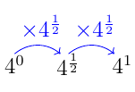
What number multiplied to itself would get us 4? 2 would work! \(2\cdot 2=4\). Note that -2 would also work since \(-2\cdot-2=4\) but in our picture, we have a positive number.

So really, the fraction in the exponent is essentially asking to do the opposite of the whole number. That is, instead of \(2^2\) asking us "what is 2 times itself twice?" we have \(4^{\frac{1}{2}}\) asking us "what number, multiplied to itself twice, will give us 4?"

What about \(27^\frac{1}{3}\)? This is asking us to find the number that when multiplied to itself 3 times, gives us 27. Well we know that \(3^3=27\) so 3 multiplied to itself 3 times gives us 27. Thus \(27^\frac{1}{3}=3\)

Example \(\PageIndex{7}\)

Compute the following

1. \(8^\frac{1}{3}\)
2. \(9^\frac{1}{2}\)
3. \(1^\frac{1}{36}\)
4. \(49^\frac{1}{2}\)

Answer

1. 2
2. 3
3. 1
4. 7

Imagine a square with all sides of the same length, say 4. The area of this is \(4\cdot 4=4^2=16\) because of this we sometimes call \(4^2\) "4 squared".

Definition: SQUARE AND SQUARE ROOT OF A NUMBER

Square

If \(n^{2}=m\), then \(m\) is the square of \(n\).

Square Root

If \(n^{2}=m\), then \(n\) is a square root of \(m\).

The square root of a number is just that number raised to the \(\frac{1}{2}\) power.

Notice \((−13)^{2} = 169\) also, so \(−13\) is also a square root of \(169\). Therefore, both \(13\) and \(−13\) are square roots of \(169\).

So, every positive number has two square roots—one positive and one negative. What if we only wanted the positive square root of a positive number? We use a radical sign, and write, \(\sqrt{m}\), which denotes the positive square root of \(m\). The positive square root is also called the principal square root.

We also use the radical sign for the square root of zero. Because \(0^{2}=0, \sqrt{0}=0\). Notice that zero has only one square root.

Definition: SQUARE ROOT NOTATION

\(\sqrt{m}\) is read "the square root of \(m\)."

If \(n^{2}=m\), then \(n=\sqrt{m}\), for \(n\geq 0\).

\[\color{cyan} \text{radical sign} \longrightarrow \color{black} \sqrt{m} \color{cyan} \longleftarrow \text{radicand} \nonumber\]

Figure 8.1.1

What about if we have \(\frac{1}{3}\) in the exponent? Is there notation for that?

Definition: N^th ROOT OF A NUMBER

If \(b^{n}=a\), then \(b\) is an \(n^{th}\) root of \(a\).

The principal \(n^{th}\) root of \(a\) is written \(\sqrt[n]{a}\).

The \(n\) is called the index of the radical.

Let's redo the last example in this notation.

Example \(\PageIndex{8}\)

Compute the following

1. \(\sqrt[3]{8}\)
2. \(\sqrt{9}\)
3. \(\sqrt[36]{1}\)
4. \(\sqrt{49}\)

Answer

1. 2
2. 3
3. 1
4. 7

What about negative numbers inside square roots? We are not ready to go there yet but we will in Chapter 4.

Example \(\PageIndex{9}\)

Simplify:

1. \(\sqrt{144}\)
2. \(-\sqrt{289}\)

Solution:

a.

\(\sqrt{144}\)

Since \(12^{2}=144\).

\(12\)

b.

\(-\sqrt{289}\)

Since \(17^{2}=289\) and the negative is in front of the radical sign.

\(-17\)

So far we have only talked about squares and square roots. Let’s now extend our vocabulary to include higher powers and higher roots.

\(\begin{array}{ll}{\text { We write: }} & {\text { We say: }} \\ {n^{2}} & {n \text { squared }} \\ {n^{3}} & {n \text { cubed }} \\ {n^{4}} & {n \text { to the fourth power }} \\ {n^{5}} & {n \text { to the fifth power }}\end{array}\)

The terms ‘squared’ and ‘cubed’ come from the formulas for area of a square and volume of a cube.

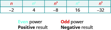
It will be helpful to have a table of the powers of the integers from \(−5\) to \(5\). See Figure 8.1.2

Figure 8.1.2

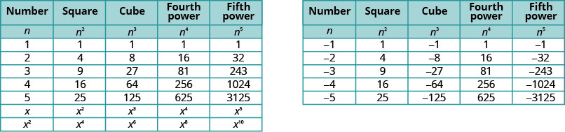
Notice the signs in the table. All powers of positive numbers are positive, of course. But when we have a negative number, the even powers are positive and the odd powers are negative. We’ll copy the row with the powers of \(−2\) to help you see this.

Figure 8.1.3

Estimate and Approximate Roots

When we see a number with a radical sign, we often don’t think about its numerical value. While we probably know that the \(\sqrt{4}=2\), what is the value of \(\sqrt{21}\) or \(\sqrt[3]{50}\)? In some situations a quick estimate is meaningful and in others it is convenient to have a decimal approximation.

To get a numerical estimate of a square root, we look for perfect square numbers closest to the radicand. To find an estimate of \(\sqrt{11}\), we see \(11\) is between perfect square numbers \(9\) and \(16\), closer to \(9\). Its square root then will be between \(3\) and \(4\), but closer to \(3\).

Figure 8.1.4

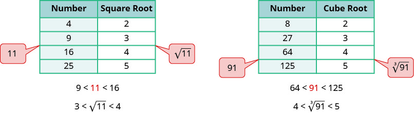
Similarly, to estimate \(\sqrt[3]{91}\), we see \(91\) is between perfect cube numbers \(64\) and \(125\). The cube root then will be between \(4\) and \(5\).

Example \(\PageIndex{10}\)

Estimate each root between two consecutive whole numbers:

1. \(\sqrt{105}\)
2. \(\sqrt[3]{43}\)

Solution:

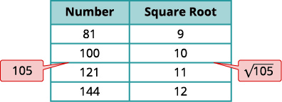
a. Think of the perfect square numbers closest to \(105\). Make a small table of these perfect squares and their squares roots.

Table 8.1.1

	\(\sqrt{105}\)
Locate \(105\) between two consecutive perfect squares.	\(100<\color{red}105 \color{black} <121\)
\(\sqrt{105}\) is between their square roots.	\(10< \color{red}\sqrt{105}< \color{black}11\)

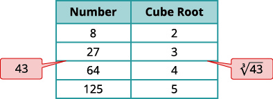
b. Similarly we locate \(43\) between two perfect cube numbers.

Table 8.1.2

	\(\sqrt[3]{43}\)
Locate \(43\) between two consecutive perfect cubes.
\(\sqrt[3]{43}\) is between their cube roots.

Exercise \(\PageIndex{11}\)

Estimate each root between two consecutive whole numbers:

1. \(\sqrt{38}\)
2. \(\sqrt[3]{93}\)

Answer

1. \(6<\sqrt{38}<7\)
2. \(4<\sqrt[3]{93}<5\)

Exercise \(\PageIndex{12}\)

Estimate each root between two consecutive whole numbers:

1. \(\sqrt{84}\)
2. \(\sqrt[3]{152}\)

Answer

1. \(9<\sqrt{84}<10\)
2. \(5<\sqrt[3]{152}<6\)

There are mathematical methods to approximate square roots, but nowadays most people use a calculator to find square roots. To find a square root you will use the \(\sqrt{x}\) key on your calculator. To find a cube root, or any root with higher index, you will use the \(\sqrt[y]{x}\) key.

When you use these keys, you get an approximate value. It is an approximation, accurate to the number of digits shown on your calculator’s display. The symbol for an approximation is \(≈\) and it is read ‘approximately’.

Suppose your calculator has a \(10\) digit display. You would see that

\(\sqrt{5} \approx 2.236067978\) rounded to two decimal places is \(\sqrt{5} \approx 2.24\)

\(\sqrt[4]{93} \approx 3.105422799\) rounded to two decimal places is \(\sqrt[4]{93} \approx 3.11\)

How do we know these values are approximations and not the exact values? Look at what happens when we square them:

\(\begin{aligned}(2.236067978)^{2} &=5.000000002 &(3.105422799)^{4}&=92.999999991 \\(2.24)^{2} &=5.0176 & (3.11)^{4}&=93.54951841 \end{aligned}\)

Their squares are close to \(5\), but are not exactly equal to \(5\). The fourth powers are close to \(93\), but not equal to \(93\).

Example \(\PageIndex{13}\)

Round to two decimal places:

1. \(\sqrt{17}\)
2. \(\sqrt[3]{49}\)
3. \(\sqrt[4]{51}\)

Solution:

a.

\(\sqrt{17}\)

Use the calculator square root key.

\(4.123105626 \dots\)

Round to two decimal places.

\(4.12\)

\(\sqrt{17} \approx 4.12\)

b.

\(\sqrt[3]{49}\)

Use the calculator \(\sqrt[y]{x}\) key.

\(3.659305710 \ldots\)

Round to two decimal places.

\(3.66\)

\(\sqrt[3]{49} \approx 3.66\)

c.

\(\sqrt[4]{51}\)

Use the calculator \(\sqrt[y]{x}\) key.

\(2.6723451177 \ldots\)

Round to two decimal places.

\(2.67\)

\(\sqrt[4]{51} \approx 2.67\)

Exercise \(\PageIndex{14}\)

Round to two decimal places:

1. \(\sqrt{11}\)
2. \(\sqrt[3]{71}\)
3. \(\sqrt[4]{127}\)

Answer

1. \(\approx 3.32\)
2. \(\approx 4.14\)
3. \(\approx 3.36\)

Exercise \(\PageIndex{15}\)

Round to two decimal places:

1. \(\sqrt{13}\)
2. \(\sqrt[3]{84}\)
3. \(\sqrt[4]{98}\)

Answer

1. \(\approx 3.61\)
2. \(\approx 4.38\)
3. \(\approx 3.15\)

Simplify Variable Expressions with Roots

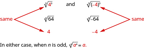
The odd root of a number can be either positive or negative. For example,

Figure 8.1.13

But what about an even root? We want the principal root, so \(\sqrt[4]{625}=5\).

But notice,

Figure 8.1.14

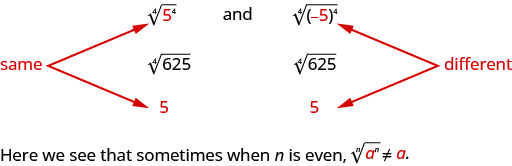
How can we make sure the fourth root of \(−5\) raised to the fourth power is \(5\)? We can use the absolute value. \(|−5|=5\). So we say that when \(n\) is even \(\sqrt[n]{a^{n}}=|a|\). This guarantees the principal root is positive.

Definition: SIMPLIFYING ODD AND EVEN ROOTS

For any integer \(n\geq 2\),

when the index \(n\) is odd \(\sqrt[n]{a^{n}}=a\)

when the index \(n\) is even \(\sqrt[n]{a^{n}}=|a|\)

We must use the absolute value signs when we take an even root of an expression with a variable in the radical.

Example \(\PageIndex{16}\)

Simplify:

1. \(\sqrt{x^{2}}\)
2. \(\sqrt[3]{n^{3}}\)
3. \(\sqrt[4]{p^{4}}\)
4. \(\sqrt[5]{y^{5}}\)

Solution:

a. We use the absolute value to be sure to get the positive root.

\(\sqrt{x^{2}}\)

Since the index \(n\) is even, \(\sqrt[n]{a^{n}}=|a|\).

b. This is an odd indexed root so there is no need for an absolute value sign.

\(\sqrt[3]{m^{3}}\)

Since the index is \(n\) is odd, \(\sqrt[n]{a^{n}}=a\).

\(m\)

c.

\(\sqrt[4]{p^{4}}\)

Since the index \(n\) is even \(\sqrt[n]{a^{n}}=|a|\).

\(|p|\)

d.

\(\sqrt[5]{y^{5}}\)

Since the index \(n\) is odd, \(\sqrt[n]{a^{n}}=a\).

\(y\)

Exercise \(\PageIndex{17}\)

Simplify:

1. \(\sqrt{b^{2}}\)
2. \(\sqrt[3]{w^{3}}\)
3. \(\sqrt[4]{m^{4}}\)
4. \(\sqrt[5]{q^{5}}\)

Answer

1. \(|b|\)
2. \(w\)
3. \(|m|\)
4. \(q\)

Exercise \(\PageIndex{18}\)

Simplify:

1. \(\sqrt{y^{2}}\)
2. \(\sqrt[3]{p^{3}}\)
3. \(\sqrt[4]{z^{4}}\)
4. \(\sqrt[5]{q^{5}}\)

Answer

1. \(|y|\)
2. \(p\)
3. \(|z|\)
4. \(q\)

What about square roots of higher powers of variables? The Power Property of Exponents says \(\left(a^{m}\right)^{n}=a^{m \cdot n}\). So if we square \(a^{m}\), the exponent will become \(2m\).

\(\left(a^{m}\right)^{2}=a^{2 m}\)

Looking now at the square root.

\(\sqrt{a^{2 m}}\)

Since \(\left(a^{m}\right)^{2}=a^{2 m}\).

\(\sqrt{\left(a^{m}\right)^{2}}\)

Since \(n\) is even \(\sqrt[n]{a^{n}}=|a|\).

\(\left|a^{m}\right|\)

So \(\sqrt{a^{2 m}}=\left|a^{m}\right|\).

We apply this concept in the next example.

Example \(\PageIndex{19}\)

Simplify:

1. \(\sqrt{x^{6}}\)
2. \(\sqrt{y^{16}}\)

Solution:

a.

\(\sqrt{x^{6}}\)

Since \(\left(x^{3}\right)^{2}=x^{6}\).

\(\sqrt{\left(x^{3}\right)^{2}}\)

Since the index \(n\) is even \(\sqrt{a^{n}}=|a|\).

\(\left|x^{3}\right|\)

b.

\(\sqrt{y^{16}}\)

Since \(\left(y^{8}\right)^{2}=y^{16}\).

\(\sqrt{\left(y^{8}\right)^{2}}\)

Since the index \(n\) is even \(\sqrt[n]{a^{n}}=|a|\).

\(y^{8}\)

In this case the absolute value sign is not needed as \(y^{8}\) is positive.

Exercise \(\PageIndex{20}\)

Simplify:

1. \(\sqrt{y^{18}}\)
2. \(\sqrt{z^{12}}\)

Answer

1. \(|y^{9}|\)
2. \(z^{6}\)

Exercise \(\PageIndex{21}\)

Simplify:

1. \(\sqrt{m^{4}}\)
2. \(\sqrt{b^{10}}\)

Answer

1. \(m^{2}\)
2. \(|b^{5}|\)

The next example uses the same idea for higher roots.

Example \(\PageIndex{22}\)

Simplify:

1. \(\sqrt[3]{y^{18}}\)
2. \(\sqrt[4]{z^{8}}\)

Solution:

a.

\(\sqrt[3]{y^{18}}\)

Since \(\left(y^{6}\right)^{3}=y^{18}\).

\(\sqrt[3]{\left(y^{6}\right)^{3}}\)

Since \(n\) is odd, \(\sqrt[n]{a^{n}}=a\).

\(y^{6}\)

b.

\(\sqrt[4]{z^{8}}\)

Since \(\left(z^{2}\right)^{4}=z^{8}\).

\(\sqrt[4]{\left(z^{2}\right)^{4}}\)

Since \(z^{2}\) is positive, we do not need an absolute value sign.

\(z^{2}\)

Exercise \(\PageIndex{23}\)

Simplify:

1. \(\sqrt[4]{u^{12}}\)
2. \(\sqrt[3]{v^{15}}\)

Answer

1. \(|u^{3}|\)
2. \(v^{5}\)

Exercise \(\PageIndex{24}\)

Simplify:

1. \(\sqrt[5]{c^{20}}\)
2. \(\sqrt[6]{d^{24}}\)

Answer

1. \(c^{4}\)
2. \(d^{4}\)

In the next example, we now have a coefficient in front of the variable. The concept \(\sqrt{a^{2 m}}=\left|a^{m}\right|\) works in much the same way.

\(\sqrt{16 r^{22}}=4\left|r^{11}\right|\) because \(\left(4 r^{11}\right)^{2}=16 r^{22}\).

But notice \(\sqrt{25 u^{8}}=5 u^{4}\) and no absolute value sign is needed as \(u^{4}\) is always positive.

Example \(\PageIndex{25}\)

Simplify:

1. \(\sqrt{16 n^{2}}\)
2. \(-\sqrt{81 c^{2}}\)

Solution:

a.

\(\sqrt{16 n^{2}}\)

Since \((4 n)^{2}=16 n^{2}\).

\(\sqrt{(4 n)^{2}}\)

Since the index \(n\) is even \(\sqrt[n]{a^{n}}=|a|\).

\(4|n|\)

b.

\(-\sqrt{81 c^{2}}\)

Since \((9 c)^{2}=81 c^{2}\).

\(-\sqrt{(9 c)^{2}}\)

Since the index \(n\) is even \(\sqrt[n]{a^{n}}=|a|\).

\(-9|c|\)

Exercise \(\PageIndex{26}\)

Simplify:

1. \(\sqrt{64 x^{2}}\)
2. \(-\sqrt{100 p^{2}}\)

Answer

1. \(8|x|\)
2. \(-10|p|\)

Exercise \(\PageIndex{27}\)

Simplify:

1. \(\sqrt{169 y^{2}}\)
2. \(-\sqrt{121 y^{2}}\)

Answer

1. \(13|y|\)
2. \(-11|y|\)

This example just takes the idea farther as it has roots of higher index.

Example \(\PageIndex{28}\)

Simplify:

1. \(\sqrt[3]{64 p^{6}}\)
2. \(\sqrt[4]{16 q^{12}}\)

Solution:

a.

\(\sqrt[3]{64 p^{6}}\)

Rewrite \(64p^{6}\) as \(\left(4 p^{2}\right)^{3}\).

\(\sqrt[3]{\left(4 p^{2}\right)^{3}}\)

Take the cube root.

\(4p^{2}\)

b.

\(\sqrt[4]{16 q^{12}}\)

Rewrite the radicand as a fourth power.

\(\sqrt[4]{\left(2 q^{3}\right)^{4}}\)

Take the fourth root.

\(2|q^{3}|\)

Exercise \(\PageIndex{29}\)

Simplify:

1. \(\sqrt[3]{27 x^{27}}\)
2. \(\sqrt[4]{81 q^{28}}\)

Answer

1. \(3x^{9}\)
2. \(3|q^{7}|\)

Exercise \(\PageIndex{30}\)

Simplify:

1. \(\sqrt[3]{125 q^{9}}\)
2. \(\sqrt[5]{243 q^{25}}\)

Answer

1. \(5p^{3}\)
2. \(3q^{5}\)

The next examples have two variables.

Example \(\PageIndex{31}\)

Simplify:

1. \(\sqrt{36 x^{2} y^{2}}\)
2. \(\sqrt{121 a^{6} b^{8}}\)
3. \(\sqrt[3]{64 p^{63} q^{9}}\)

Solution:

a.

\(\sqrt{36 x^{2} y^{2}}\)

Since \((6 x y)^{2}=36 x^{2} y^{2}\)

\(\sqrt{(6 x y)^{2}}\)

Take the square root.

\(6|xy|\)

b.

\(\sqrt{121 a^{6} b^{8}}\)

Since \(\left(11 a^{3} b^{4}\right)^{2}=121 a^{6} b^{8}\)

\(\sqrt{\left(11 a^{3} b^{4}\right)^{2}}\)

Take the square root.

\(11\left|a^{3}\right| b^{4}\)

c.

\(\sqrt[3]{64 p^{63} q^{9}}\)

Since \(\left(4 p^{21} q^{3}\right)^{3}=64 p^{63} q^{9}\)

\(\sqrt[3]{\left(4 p^{21} q^{3}\right)^{3}}\)

Take the cube root.

\(4p^{21}q^{3}\)

Exercise \(\PageIndex{32}\)

Simplify:

1. \(\sqrt{100 a^{2} b^{2}}\)
2. \(\sqrt{144 p^{12} q^{20}}\)
3. \(\sqrt[3]{8 x^{30} y^{12}}\)

Answer

1. \(10|ab|\)
2. \(12p^{6}q^{10}\)
3. \(2x^{10}y^{4}\)

Exercise \(\PageIndex{33}\)

Simplify:

1. \(\sqrt{225 m^{2} n^{2}}\)
2. \(\sqrt{169 x^{10} y^{14}}\)
3. \(\sqrt[3]{27 w^{36} z^{15}}\)

Answer

1. \(15|mn|\)
2. \(13\left|x^{5} y^{7}\right|\)
3. \(3w^{12}z^{5}\)

Access this online resource for additional instruction and practice with simplifying expressions with roots.

• Simplifying Variables Exponents with Roots using Absolute Values

Key Concepts

• Square Root Notation
  • \(\sqrt{m}\) is read ‘the square root of \(m\)’
  • If \(n^{2}=m\), then \(n=\sqrt{m}\), for \(n≥0\).
    
    Figure 8.1.1
  • The square root of \(m\), \(\sqrt{m}\), is a positive number whose square is \(m\).
• n^th Root of a Number
  • If \(b^{n}=a\), then \(b\) is an \(n^{th}\) root of \(a\).
  • The principal \(n^{th}\) root of \(a\) is written \(\sqrt[n]{a}\).
  • \(n\) is called the index of the radical.
• Properties of \(\sqrt[n]{a}\)
  • When \(n\) is an even number and
    • \(a≥0\), then \(\sqrt[n]{a}\) is a real number
    • \(a<0\), then \(\sqrt[n]{a}\) is not a real number
  • When \(n\) is an odd number, \(\sqrt[n]{a}\) is a real number for all values of \(a\).
• Simplifying Odd and Even Roots
  • For any integer \(n≥2\),
    • when \(n\) is odd \(\sqrt[n]{a^{n}}=a\)
    • when \(n\) is even \(\sqrt[n]{a^{n}}=|a|\)
  • We must use the absolute value signs when we take an even root of an expression with a variable in the radical.

Glossary

square of a number

If \(n^{2}=m\), then \(m\) is the square of \(n\).

square root of a number

If \(n^{2}=m\), then \(n\) is a square root of \(m\).