
4.6E: Exercises
- Page ID
- 108361
\( \newcommand{\vecs}[1]{\overset { \scriptstyle \rightharpoonup} {\mathbf{#1}} } \) \( \newcommand{\vecd}[1]{\overset{-\!-\!\rightharpoonup}{\vphantom{a}\smash {#1}}} \)\(\newcommand{\id}{\mathrm{id}}\) \( \newcommand{\Span}{\mathrm{span}}\) \( \newcommand{\kernel}{\mathrm{null}\,}\) \( \newcommand{\range}{\mathrm{range}\,}\) \( \newcommand{\RealPart}{\mathrm{Re}}\) \( \newcommand{\ImaginaryPart}{\mathrm{Im}}\) \( \newcommand{\Argument}{\mathrm{Arg}}\) \( \newcommand{\norm}[1]{\| #1 \|}\) \( \newcommand{\inner}[2]{\langle #1, #2 \rangle}\) \( \newcommand{\Span}{\mathrm{span}}\) \(\newcommand{\id}{\mathrm{id}}\) \( \newcommand{\Span}{\mathrm{span}}\) \( \newcommand{\kernel}{\mathrm{null}\,}\) \( \newcommand{\range}{\mathrm{range}\,}\) \( \newcommand{\RealPart}{\mathrm{Re}}\) \( \newcommand{\ImaginaryPart}{\mathrm{Im}}\) \( \newcommand{\Argument}{\mathrm{Arg}}\) \( \newcommand{\norm}[1]{\| #1 \|}\) \( \newcommand{\inner}[2]{\langle #1, #2 \rangle}\) \( \newcommand{\Span}{\mathrm{span}}\)\(\newcommand{\AA}{\unicode[.8,0]{x212B}}\)
Practice Makes Perfect
In the following exercises, graph the functions by plotting points.
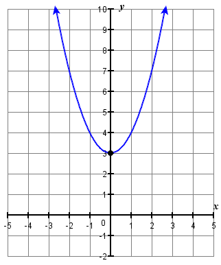
- \(f(x)=x^{2}+3\)
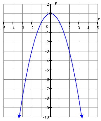
- \(y=-x^{2}+1\)
- Answer
-
1.
2.
For each of the following exercises, determine if the parabola opens up or down.
3. a. \(f(x)=-2 x^{2}-6 x-7\) b. \(f(x)=6 x^{2}+2 x+3\)
4. a. \(f(x)=-3 x^{2}+5 x-1\) b. \(f(x)=2 x^{2}-4 x+5\)
- Answer
-
3. a. down b. up
4. a. down b. up
In the following functions, find
- The equation of the axis of symmetry
- The vertex of its graph
- \(f(x)=x^{2}+8 x-1\)
- \(f(x)=x^{2}+10 x+25\)
- \(f(x)=-x^{2}+2 x+5\)
- \(f(x)=-2 x^{2}-8 x-3\)
- Answer
-
- a. Axis of symmetry: \(x=-4\) b. Vertex: \((-4,-17)\)
- a. Axis of symmetry: \(x=-5\) b. Vertex: \((-5,0)\)
- a. Axis of symmetry: \(x=1\) b. Vertex: \((1,6)\)
- a. Axis of symmetry: \(x=-2\) b. Vertex: \((-2,5)\)
In the following exercises, find the intercepts of the parabola whose function is given.
- \(f(x)=x^{2}+7 x+6\)
- \(f(x)=x^{2}+8 x+12\)
- \(f(x)=-x^{2}+8 x-19\)
- \(f(x)=x^{2}+6 x+13\)
- \(f(x)=4 x^{2}-20 x+25\)
- \(f(x)=-x^{2}-6 x-9\)
- Answer
-
- \(y\)-intercept: \((0,6)\); \(x\)-intercept(s): \((-1,0), (-6,0)\)
- \(y\)-intercept: \((0,12)\); \(x\)-intercept(s): \((-2,0), (-6,0)\)
- \(y\)-intercept: \((0,-19)\); \(x\)-intercept(s): none
- \(y\)-intercept: \((0,13)\); \(x\)-intercept(s): none
- \(y\)-intercept: \((0,25)\); \(x\)-intercept(s): \((\frac{5}{2},0)\)
- \(y\)-intercept: \((0,-9)\); \(x\)-intercept(s): \((-3,0)\)
In the following exercises, graph the function by using its properties. That is, find its \(x\)-intercepts, \(y\)-intercept, vertex, and determine its end behavior. Then use this information to graph the function.
- \(f(x)=x^{2}+6 x+5\)
- \(f(x)=x^{2}+4 x+3\)
- \(f(x)=9 x^{2}+12 x+4\)
- \(f(x)=-x^{2}+2 x-7\)
- \(f(x)=2 x^{2}-4 x+1\)
- \(f(x)=2 x^{2}-4 x+2\)
- \(f(x)=-x^{2}-4 x+2\)
- \(f(x)=5 x^{2}-10 x+8\)
- \(f(x)=3 x^{2}+18 x+20\)
- Answer
-
15.
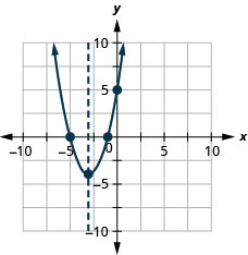
Figure 9.6.136 16.
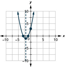
Figure 9.6.137 17.
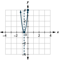
Figure 9.6.138 18.
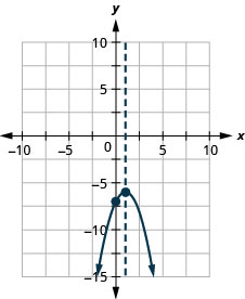
Figure 9.6.139 19.
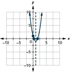
Figure 9.6.140 20.
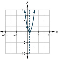
Figure 9.6.141 21.
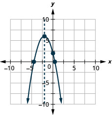
Figure 9.6.142 22.
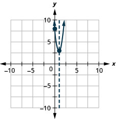
Figure 9.6.143 23.
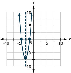
Figure 9.6.144