22.7: J1.07- Section 2 Example 6

Last updated
Save as PDF

Page ID: 51730

$ \newcommand{\vecs}[1]{\overset { \scriptstyle \rightharpoonup} {\mathbf{#1}} } $ $ \newcommand{\vecd}[1]{\overset{-\!-\!\rightharpoonup}{\vphantom{a}\smash {#1}}} $$\newcommand{\id}{\mathrm{id}}$ $ \newcommand{\Span}{\mathrm{span}}$ $ \newcommand{\kernel}{\mathrm{null}\,}$ $ \newcommand{\range}{\mathrm{range}\,}$ $ \newcommand{\RealPart}{\mathrm{Re}}$ $ \newcommand{\ImaginaryPart}{\mathrm{Im}}$ $ \newcommand{\Argument}{\mathrm{Arg}}$ $ \newcommand{\norm}[1]{\| #1 \|}$ $ \newcommand{\inner}[2]{\langle #1, #2 \rangle}$ $ \newcommand{\Span}{\mathrm{span}}$ $\newcommand{\id}{\mathrm{id}}$ $ \newcommand{\Span}{\mathrm{span}}$ $ \newcommand{\kernel}{\mathrm{null}\,}$ $ \newcommand{\range}{\mathrm{range}\,}$ $ \newcommand{\RealPart}{\mathrm{Re}}$ $ \newcommand{\ImaginaryPart}{\mathrm{Im}}$ $ \newcommand{\Argument}{\mathrm{Arg}}$ $ \newcommand{\norm}[1]{\| #1 \|}$ $ \newcommand{\inner}[2]{\langle #1, #2 \rangle}$ $ \newcommand{\Span}{\mathrm{span}}$$\newcommand{\AA}{\unicode[.8,0]{x212B}}$

Example 6: Comparing different models of sales-data history (when both fit the data)

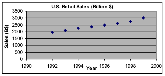
The dataset below of total retail sales in the United States from 1992 to 1999 looks as if it could be fit pretty closely by a linear model, in which sales increase by the same amount each year. However, most economic trends increase by about the same percentage each year on the average, so an exponential model might be more appropriate and would also be a good fit. To choose between these alternatives, we will find both best-fit models and examine what happens to them when extrapolated back 20 years.

Year	Sales (B$)
1992	1,952
1993	2,082
1994	2,248
1995	2,359
1996	2,502
1997	2,611
1998	2,746
1999	2,995

$1$

Question: For this data, which model has more reasonable extrapolation behavior—linear or exponential?

Solution approach:

[1] Copy the dataset into the Data Scratch Pad worksheet in Models.xls and modify it so that the input variable is years since 1992. This will make the model parameters easier to find. (The redefined dataset is shown to the right.)

[2] Use a copy of the Linear Model template to find the best linear model, which is about $y=141x+1943$

[3] Use the Exponential Model template to find the best exponential model, which is about $y=1971\cdot{{(1.06)}^{x}}$

[5] Note that the graphs of the two models both fit the data well.

Since 1992	Sales (B$)
0	1,952
1	2,082
2	2,248
3	2,359
4	2,502
5	2,611
6	2,746
7	2,995

In both the Linear Model and Exponential Model worksheets, follow these steps:

[a] Insert the values from -1 to -20 into column A below the existing data. These new input values correspond to the years from 1991 back to 1972. [6] In both the Linear Model and Exponential Model worksheets, follow these steps:

[b] Spread the formula in column C down as far as the new input values. This will give the sales prediction of that model for the previous 20 years. The results for the two models should look like the worksheet extracts shown below.

Extracts from Models.xls worksheets, with extrapolations back for 20 years

Linear Model $y=141x+1943$

	A	B	C
1	x	y data	y model
2	Year-1992	Sales (B$)	Prediction
3	0	1,952	1943
4	1	2,082	2084
5	2	2,248	2225
6	3	2,359	2366
7	4	2,502	2507
8	5	2,611	2648
9	6	2,746	2789
10	7	2,995	2930
11	-1		1802
12	-2		1661
13	-3		1520
14	-4		1379
15	-5		1238
16	-6		1097
17	-7		956
18	-8		815
19	-9		674
20	-10		533
21	-11		392
22	-12		251
23	-13		110
24	-14		-31
25	-15		-172
26	-16		-313
27	-17		-454
28	-18		-595
29	-19		-736
30	-20		-877

Exponential Model $y=1971\cdot{{(1+0.06)}^{x}}$

	A	B	C
1	x	y data	y model
2	Year-1992	Sales (B$)	Prediction
3	0	1,952	1971.00
4	1	2,082	2089.26
5	2	2,248	2214.62
6	3	2,359	2347.49
7	4	2,502	2488.34
8	5	2,611	2637.64
9	6	2,746	2795.90
10	7	2,995	2963.66
11	-1		1859.43
12	-2		1754.18
13	-3		1654.89
14	-4		1561.22
15	-5		1472.85
16	-6		1389.48
17	-7		1310.83
18	-8		1236.63
19	-9		1166.63
20	-10		1100.60
21	-11		1038.30
22	-12		979.53
23	-13		924.08
24	-14		871.78
25	-15		822.43
26	-16		775.88
27	-17		731.96
28	-18		690.53
29	-19		651.44
30	-20		614.57

[c] Make a new graph of the data and model (the A1:C30 rectangle of cells). In the graphs below showing the extrapolations, the scales have been set to equal and gridlines have been omitted, to make comparisons easier. But default-setting graphs will have the same information.

[6] Compare the extrapolated models. In this case, the linear extrapolation back 20 years predicts negative sales totals in 1972, which is obviously unrealistic. The exponential model remains positive regardless of how far back it is extrapolated, which shows that the exponential model is a much better choice for a sales model.

Mathematics for Modeling. Authored by: Mary Parker and Hunter Ellinger. License: CC BY: Attribution