11.12: Regression and Correlation

Last updated
Save as PDF

Page ID: 51632

$ \newcommand{\vecs}[1]{\overset { \scriptstyle \rightharpoonup} {\mathbf{#1}} } $ $ \newcommand{\vecd}[1]{\overset{-\!-\!\rightharpoonup}{\vphantom{a}\smash {#1}}} $$\newcommand{\id}{\mathrm{id}}$ $ \newcommand{\Span}{\mathrm{span}}$ $ \newcommand{\kernel}{\mathrm{null}\,}$ $ \newcommand{\range}{\mathrm{range}\,}$ $ \newcommand{\RealPart}{\mathrm{Re}}$ $ \newcommand{\ImaginaryPart}{\mathrm{Im}}$ $ \newcommand{\Argument}{\mathrm{Arg}}$ $ \newcommand{\norm}[1]{\| #1 \|}$ $ \newcommand{\inner}[2]{\langle #1, #2 \rangle}$ $ \newcommand{\Span}{\mathrm{span}}$ $\newcommand{\id}{\mathrm{id}}$ $ \newcommand{\Span}{\mathrm{span}}$ $ \newcommand{\kernel}{\mathrm{null}\,}$ $ \newcommand{\range}{\mathrm{range}\,}$ $ \newcommand{\RealPart}{\mathrm{Re}}$ $ \newcommand{\ImaginaryPart}{\mathrm{Im}}$ $ \newcommand{\Argument}{\mathrm{Arg}}$ $ \newcommand{\norm}[1]{\| #1 \|}$ $ \newcommand{\inner}[2]{\langle #1, #2 \rangle}$ $ \newcommand{\Span}{\mathrm{span}}$$\newcommand{\AA}{\unicode[.8,0]{x212B}}$

Objective

Here you will learn about pairs of variables that are related in a linear fashion, including those with values occurring
in a slightly random manner.
Here you will learn to calculate the linear correlation coefficient, and how to use it to describe the relationship between an explanatory and response variable.

Linear Relationships

Imagine walking through the electronics section of your local department store. On the wall are examples of dozens of television sets, from little 1900 units made to sit on a kitchen counter to 72″+ monsters meant to be the centerpiece of a home theatre. Looking at the prices, you note without surprise that the 72″ model is more expensive than the 19″, and a 42″ model is priced in between. It seems rather clear that as the TV gets larger, the price goes up. Does that mean increased screen size causes increased price?

$BestBuy$

Look to the end of the section for the answer.

Watch This: Exploring Linear Relationships

$Thumbnail for the embedded element "Modeling with linear equations example 1 | Linear equations and functions | 8th grade | Khan Academy"$

A YouTube element has been excluded from this version of the text. You can view it online here: http://pb.libretexts.org/mala/?p=160

When two quantities are compared, it is not uncommon to note a relationship between them that indicates both quantities increase and decrease at the same time, or that one increases as the other decreases. If both quantities are plotted on coordinate axes, the data points show a general or definite linear trend.

If the points actually form a clearly defined line, the variables may be an example of a deterministic relationship. A deterministic relationship indicates that the value of one variable can be reliably and accurately determined by the manipulation of the other variable. An example might be inches and centimeters: one inch is the same as 2.54 centimeters. If you know how many inches long something is, you can reliably and accurately calculate the number of centimeters long the same item is.

As you likely recall from Algebra, the slope describes the angle of the line created by plotting points from a linear relationship, and the point where the explanatory variable has a value of zero is called the y-intercept (commonly denoted b).

Often, particularly in research situations when one or both variables are measured, the plotted values are generally linear, but do not line up precisely. When two variables seem to show a linear relationship, but the values display some amount of randomness, we commonly visually describe the relationship with a scatter plot. As you will see throughout this chapter, the strength of the linear relationship of the variables can be described through mathematics.

Example 1

Given the equation y = 2.3x + 5:

Create an x–y table to describe the values of at least four points
What is the slope of the line?
What is the y-intercept?

Solution

Pick a value for x, substitute the chosen value for x in the equation, and calculate y:
Table 1

x calculation y

1 y = 2.3(1) + 5 7.3

2 y = 2.3(2) + 5 9.6

0 y = 2.3(0) + 5 5

−1 y = 2.3(−1) + 5 2.7

The equation in the problem is in y = mx + b form (also known as slope-intercept form), where b is the y-value when x = 0, and m is the slope of the line.
m = 2.3
b = 5

Table 1
x	calculation	y
1	y = 2.3(1) + 5	7.3
2	y = 2.3(2) + 5	9.6
0	y = 2.3(0) + 5	5
−1	y = 2.3(−1) + 5	2.7

Example 2

Given the equation y = −3x + 3.9:

Create an x–y table to describe the values of at least four points
What is the slope of the line?
What is the y-intercept?

Solution

Pick a value for x, substitute the chosen value for x in the equation, and calculate y:
Table 2

x calculation y

1 y = −3(1) + 3.9 6.9

2 y = −3(2) + 3.9 9.9

0 y = −3(0) + 3.9 3.9

−1 y = −3(−1) + 3.9 0.9

The equation in the problem is in y = mx + b form (also known as slope-intercept form), where b is the y-value when x = 0, and m is the slope of the line.
m = −3
b = 3.9

Table 2
x	calculation	y
1	y = −3(1) + 3.9	6.9
2	y = −3(2) + 3.9	9.9
0	y = −3(0) + 3.9	3.9
−1	y = −3(−1) + 3.9	0.9

Example 3

Given the equation y = −2.8x − 9.1:

Create an x–y table to describe the values of at least four points.
What is the slope of the line?
What is the y-intercept?

Solution

Pick a value for x, substitute the chosen value for x in the equation, and calculate y:
Table 3

x calculation y

1 y = −2.8(1) − 9.1 −11.9

2 y = −2.8(2) − 9.1 −14.7

0 y = −2.8(0) − 9.1 −9.1

−1 y = −2.8(−1) − 9.1 6.3

The equation in the problem is in y = mx + b form (also known as slope-intercept form), where b is the y-value when x = 0, and m is the slope of the line.
m = −2.8
b = −9.1

Table 3
x	calculation	y
1	y = −2.8(1) − 9.1	−11.9
2	y = −2.8(2) − 9.1	−14.7
0	y = −2.8(0) − 9.1	−9.1
−1	y = −2.8(−1) − 9.1	6.3

Intro Problem Revisited

No, it does not. This is an example of the difficulty associated with examining linear relationships. Correlation does not imply causation. Just because a pair of variables exhibit a relationship, linear or otherwise, does not mean that one variable causes changes in the other variable.

Vocabulary

Cartesian Graph: a “plus-shaped” graph, with the explanatory variable (the input value) plotted horizontally on the x-axis, and the response variable (the output value) plotted vertically on the y-axis.

Deterministic linear relationship: a relationship that plots a reliably straight and accurate single line.

Slope of a line: (commonly denoted m) describes the angle of a plotted line on a graph.

Scatter plot: a graph of individual points on an x–y graph.

Guided Practice

If a linear graph exhibits a positive slope, what can you predict will happen to the response variable as the explanatory variable increases?
If a linear graph has no slope, what does that mean?
Given the linear equation 2y = 5.2x + 7:
1. What is the slope?
2. What is the y-interept?
3. What happens to y as x increases?
Given the equation y = 2x² +4:
1. Is this a linear equation? Why or why not?
2. Does this equation represent a relationship?

Solutions

A positive slope indicates that the variables increase and decrease together.
A line with no slope is a horizontal line, since the only defined variable is the output. No matter what value is given for the explanatory variable, the response is the same.
Answers:
1. The slope, m, is 5.2.
2. The y-intercept, b, is 7.
3. Since this line has a positive slope, y increases as x increases.
Answers:
1. No, the explanatory variable is squared, this graph would form a parabola.
2. Yes! It is just not a linear relationship.

Linear Correlation Coefficient

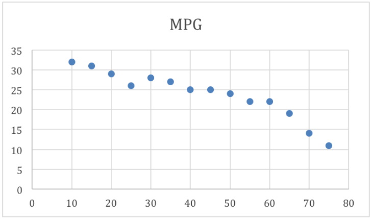
Suppose you have noted that your car seems to use more gas when you drive fast than when you drive more slowly. You decide to see how strong the relationship is, so you do some research, collect the data, and plot the data on the graph below, where the explanatory variable x is mph, and the response variable y is mpg. How can you describe how strong the correlation is without the graph?

$Fig5_4_1$

Watch This: The Correlation Coefficient and Coefficient of Determination

$Thumbnail for the embedded element "The Correlation Coefficient and Coefficient of Determination (Old, fast version)"$

A YouTube element has been excluded from this version of the text. You can view it online here: http://pb.libretexts.org/mala/?p=160

The linear correlation coefficient (sometimes called Pearson’s Correlation Coefficient), commonly denoted r, is a measure of the strength of the linear relationship between two variables. The value of r has the following properties:

r is always a value between −1 and +1
The further an r value is from zero, the stronger the relationship between the two variables.
The sign of r indicates the nature of the relationship: A positive r indicates a positive relationship, and a negative r indicates a negative relationship.

Generally speaking, you may think of the values of r in the following manner:

If |r| is between 0.85 and 1, there is a strong correlation.
If |r| is between 0.5 and 0.85, there is a moderate correlation.
If |r| is between 0.1 and 0.5, there is a weak correlation.
If |r| is less than 0.1, there is no apparent correlation.

Naturally, r-value can be calculated, but the formula is a bit beyond the scope of this course. Fortunately, there are many excellent and free online calculators for determining the r-value of a set of data. In this reading, I will be using the one at easycalculation.com, but a search for “correlation calculator online” will yield the most current options.

At the risk of overloading you with new terms, there is one more that I think it is worth learning in this reading, the coefficient of determination. The coefficient of determination is very simple to calculate if you know the correlation coefficient, since it is just r². The reason I mention it is that the coefficient of determination can be interpreted as the percentage of variation of the y variable that can be attributed to the relationship. In other words, a value of r² = .63 can be interpreted as “63% of the changes between one y value and another can be attributed to y’s relationship with x.”

Example 4

Elaina is curious about the relationship between the weight of a dog and the amount of food it eats. Specifically, she wonders if heavier dogs eat more food, or if age and size factor in. She works at the Humane Society, and does some research. After some calculation, she determines that dog weight and food weight exhibit an r-value of 0.73.

$3721602063_2aff52e447_z$

What can Elaina say about the relationship, based on her research? What percentage of the increases in food intake can she attribute to weight, according to her research?

Solution

The calculated r-value of 0.73 tells us that Elaina’s data demonstrates a moderate to strong correlation between the variables.

Since the coefficient of determination tells us the percentage of changes in the output variable that can be attributed to the input variable, we need to calculate r²:

r² = (0.73)² = .5329

Approximately 53% of increases in food intake can be attributed to the linear relationship between food intake and the weight of the dog, suggesting that other factors, perhaps age and size, are also involved.

Example 5

Tuscany wonders if barrel racing times are related to the age of the horse. Specifically, she wonders if older horses take longer to complete a barrel racing run. As a member of the Pony Club, she does some research, and determines that horse age to barrel run time exhibits an r-value of 0.52.

What can Tuscany say about horse age vs barrel race time, according to her research?

Solution

Tuscany’s research suggests that there is a moderate to weak correlation between horse age and barrel run time. In other words, the research suggests that (0.52)² = .27 = 27% of the differences between barrel run times could be attributable to the linear relationship between barrel run time and the age of the horse.

Example 6

Sayber has collected the following data regarding player score vs age in his favorite online game. He suspects that increased age is not a good indicator of gaming ability. What are the linear correlation coefficient and coefficient of determination values of his data, and how do they support or not support Sayber’s hypothesis?

Table 4
Age	Avg. Player Score
12	5,120
14	6,328
18	7,892
22	7,340
28	6,987
34	7,750
42	5,421

Solution

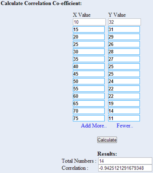
Let’s use the online calculator at easycalculation.com for this one.

I entered the explanatory (Age) and response (Player Score) values into the calculator:

$Fig5_4_2$

The linear correlation coefficient of approximately 0.04 suggests that there is no appreciable linear correlation. The coefficient of determination of 0.0016 suggests that perhaps 0.16% (practically none) of the variability of the player score is dependent on age.

Looking at the scores, however, something seems a miss with our findings. The scores suggest that age has no bearing on player score, but look at the graph of the same data:

$Fig5_4_3$

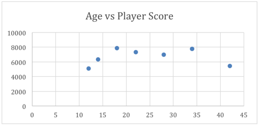
The graph suggests that the youngest and oldest polled players score less than players in late teens to mid-thirties, which seems reasonable.

This is an important example of the weakness of using just one indicator of the relationship between two variables. As I noted early in the reading, the r-value is only an indicator of linear correlation, it says nothing at all about other kinds of variable relationships. It is always a good idea to review your data in different ways to evaluate your initial conclusions.

Intro Problem Revisited

$Fig5_4_4$

After the reading above, we know that the r-value or r²-value of the relationship between MPG and MPH would describe the strength of the linear relationship in a single value.

By taking the data points detailed on the graph (in practice, of course, I would have had them in table format already, since I would have needed them to build the graph in the first place), and entering them into a free linear coefficient calculator online, I get an r-value of −0.943, indicating a strong negative relationship. This also translates into an r²-value of (−0.943)² = 0.89, indicating that the research suggests that approximately 89% of the decrease in MPG from left to right across the graph can be attributed to the increase in MPH.

Vocabulary

Linear correlation coefficient or r-value of a relationship: describes the strength of the linear relationship.

Coefficient of determination or r²-value of a relationship: indicates the approximate percentage of variation in the response variable that can be attributed to the linear relationship between the response and explanatory variables, according to the data presented.

Guided Practice

What can you say about the strength of a linear relationship with an r-value of −0.87?
What can you say about the level of negative correlation of a relationship if you know the coefficient of determination is 0.82?
How much of the variability of y is attributable to x in a relationship with an r-value of 0.76?

Solutions

An |r| of > 0.85 indicates a strong linear relationship. The fact that r is negative indicates that as x increases, y decreases.
Nothing! The coefficient of determination is r², and therefore always positive. We know that |r|= $\sqrt{.82}\approx{.91}\\$ , so this is a strong linear correlation, but we have no idea if it is positive or negative.
The coefficient of determination describes the variation in y attributable to x, so we need to find r²: (0.76)2 = .5776. Approximately 57.76% of the change in y-values can be attributed to the change in x.

Practice Questions

For the following questions, find the x and y intercepts of the given equations.

−x + 4y = 8
3x + 5y = 15
−3x + 4y = 36
−8x + 5y = 40
5x − 6y = −30
−9x − 3y = −54
−x + 5y = −10
−3x + 8y = −72

For the following questions, graph the line.

x + 3y = 2
m = −4, b = $\frac{4}{3}\\$
x-intercept = −1, y-intercept = 2
y = −4x + 2
m = −1, b = $\frac{1}{2}\\$
x + 2y = 5
−3x + 2y = −3

For the following questions, describe the relationship based on the r-value.

r = 0
r = 0.91
r = −0.49
r = 0.05
r = 1

For the following questions, describe the relationship based on the coefficient of determination:

r² = 0.82
r² = 0.15
r² = 0.47
r² = 1
r²= 0

The following questions refer to the data in the following table:

Table 5
x	y
5	70
7	69
13	58
22	47
36	36
38	25
45	14

What is the linear correlation coefficient of the data?
What does r tell you about the relationship?
What is the r² value of the data?
What does the coefficient of determination tell you about this relationship?
What would a graph of the data look like?

Regression and Correlation. Authored by: Karen Walters. Provided by: CK-12 Foundation. Located at: http://www.ck12.org/. License: CC BY-NC: Attribution-NonCommercial
Best Buy section QR codes. Authored by: Eliot Phillips. Located at: https://flic.kr/p/98ookU. License: CC BY-NC: Attribution-NonCommercial
Puppies eating. Authored by: Christian Haugen. Located at: https://flic.kr/p/6ESbCP. License: CC BY: Attribution

The Correlation Coefficient and Coefficient of Determination (Old, fast version). Authored by: jbstatistics. Located at: https://youtu.be/dCgIavyFWIo. License: All Rights Reserved. License Terms: Standard YouTube License