18.2: L1.03- Section 2

Last updated
Save as PDF

Page ID: 51695

$ \newcommand{\vecs}[1]{\overset { \scriptstyle \rightharpoonup} {\mathbf{#1}} } $ $ \newcommand{\vecd}[1]{\overset{-\!-\!\rightharpoonup}{\vphantom{a}\smash {#1}}} $$\newcommand{\id}{\mathrm{id}}$ $ \newcommand{\Span}{\mathrm{span}}$ $ \newcommand{\kernel}{\mathrm{null}\,}$ $ \newcommand{\range}{\mathrm{range}\,}$ $ \newcommand{\RealPart}{\mathrm{Re}}$ $ \newcommand{\ImaginaryPart}{\mathrm{Im}}$ $ \newcommand{\Argument}{\mathrm{Arg}}$ $ \newcommand{\norm}[1]{\| #1 \|}$ $ \newcommand{\inner}[2]{\langle #1, #2 \rangle}$ $ \newcommand{\Span}{\mathrm{span}}$ $\newcommand{\id}{\mathrm{id}}$ $ \newcommand{\Span}{\mathrm{span}}$ $ \newcommand{\kernel}{\mathrm{null}\,}$ $ \newcommand{\range}{\mathrm{range}\,}$ $ \newcommand{\RealPart}{\mathrm{Re}}$ $ \newcommand{\ImaginaryPart}{\mathrm{Im}}$ $ \newcommand{\Argument}{\mathrm{Arg}}$ $ \newcommand{\norm}[1]{\| #1 \|}$ $ \newcommand{\inner}[2]{\langle #1, #2 \rangle}$ $ \newcommand{\Span}{\mathrm{span}}$$\newcommand{\AA}{\unicode[.8,0]{x212B}}$

Section 2: Using Solver in the Tool menu to find the best-fit parameters for a model

The “Solver” add-in can be used with an appropriately-formatted spreadsheet to tell the computer to do automatically what you did by hand in the earlier model-fitting exercises – adjust the parameters until the model is a good as it can be. Solver uses the numerical value of the sum-of-squared-deviations indicator (computed in cell H8 in the example spreadsheet) to decide on the best parameters.

When you use Solver for modeling, you will set up a modeling worksheet exactly as the previous example, then use Solver to tell the computer to minimize the cell containing the goodness-of-fit indicator by adjusting the cells containing the parameters. The software then systematically searches for the parameter settings that result in the smallest standard deviation.

The Solver routine does not know anything about modeling — it simply changes the numbers in the cells you identify (G3 and G4 in this case), searching for values that produce the result you ask for (minimization) in the target cell that you identify (H8). This procedure finds the best model because of the way the worksheet is set up, with the sequence of connections where the parameters in column G are used in the model formulas in column C, which determine the data-model deviations in column D and thus the squared deviations in column E, which are added to form the sum of squared deviations indicator.

Since Solver will default to the last values used, once you start using it you will often find that the settings are already correct, so that you can just press “Solve” to get the best-fit model parameters for the current set of data. If the computer does not find a solution when fitting a model, this usually means that you forgot to set the “Min” option, so that the program is instead trying to find a maximum, an impossible task in this case because there is no limit to how far away the model can get from the data.

Usually Solver will find a correct solution regardless of the initial values of the parameters. However, it will be more dependable if you start with the parameters having values that put the model graph in the same general region as the data points. Otherwise the formula may have a value so large or small that the computer cannot handle it correctly. In any case, it is important to look at the graph of the fitted values to make sure Solver worked correctly—after the computer does the tedious part, it’s your turn to do the thinking that is needed.

Example 3: Use Solver to find the formula of the best-fit exponential model for the worksheet modified in Example 1 to include a sum-of-square deviations value.

Select the cell containing the sum-of-squared-deviations value (cell H8).
Select Solver from the Tools menu (if it is not there, select Add-Ins and add it). The dialog box should show the selected cell (e.g., “H8”) in the Set Target Cell section at the top. If not, enter it.
Choose the “Min” (for Minimum) option in the second line, since we want Solver to find the smallest possible value for the indicator in H8.
Enter “G3,G4” into the “By Changing Cells” section on the fourth line. This tells Solver to adjust the cells that we are using as model parameters when it is trying to minimize H8.
Press the “Solve” button at top right.
Check the graph (or the numbers in columns B and C) to see if the model now is close to the data, with some on each side. If it is not, you have made a mistake and must repeat the process correctly.
If the graph is acceptable, press “OK” to accept the solution that is found. The parameters (and thus the “Model” values in the column C) are now set to the best-fit values to a very high accuracy.

[reveal-answer q=”126306″]Show Answer[/reveal-answer]
[hidden-answer a=”126306″]

The best-fit exponential model formula for this data is $y=3.11\cdot{{(1.0289)}^{x}}$ (with the parameters rounded off to 3 digits to match the data). The sum of squared deviations for this model is about 1.72, which is only 53% of the 3.24 value found by hand in the previous example, and only 35% of the value for the parameter setting we originally found by visual inspection.

	A	B	C	D	E	F	G	H	I
1	x	data y	model y	Data-Model	Squared	Exponential model: y = a (1+r)^x*
2	Year-1780	Population	Prediction	deviation	deviation		y = 3.108069 * (1.028937^x)
3	0	2.8	3.108101	-0.308101	0.094926		3.108069	a: Initial value at x=0
4	10	3.9	4.134104	-0.234104	0.054804		0.028937	r: Growth rate
5	20	5.3	5.498797	-0.198797	0.039520
6	30	7.2	7.313983	-0.113983	0.012992
7	40	9.6	9.728374	-0.128374	0.016480		*Goodness of fit for these settings*
8	50	12.9	12.93977	-0.039770	0.001582	Sum of sq. dev.		1.721981
9	60	17.1	17.21127	-0.111268	0.012381
10	70	23.2	22.89281	0.307187	0.094364
11	80	31.4	30.44987	0.950128	0.902744
12	90	39.8	40.50156	-0.701561	0.492188

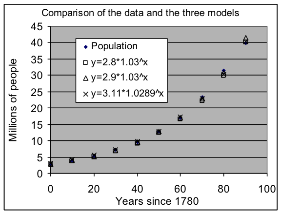
Note that the best-fit model has a starting value that is a bit higher than in the earlier models (3.11 instead of 2.8 or 2.9), but this is balanced by the growth rate being slightly lower (0.0289 instead of 0.03).

Also note that the graphs of all three models are quite close to the data, so that any could be considered a good model, and it would not be feasible to choose between them visually.

$graph1$

Example 4: Use Solver to find the best-fit linear model for the sediment depth data from the topic on linear modeling.

Solution approach:

[a] Use a spreadsheet as before, but now add the squared deviations into column E and compute their sum with a formula in G11, then use Solver to find the best-fit parameter settings.

[b] Write the linear equation with those parameters used as intercept and slope values.

[reveal-answer q=”715980″]Show Answer[/reveal-answer]
[hidden-answer a=”715980″]

The best-fit linear model to the sediment data is $y=1.759x+12.657$ .

	A	B	C	D	E	F	G
1	x	y data	y model	Residual	Squared		Linear model: y = m x + b*
2	Days	Depth	Prediction	deviation	deviation		y = 1.759286 x + 12.65714
3	10	29.9	30.25	-0.35	0.1225		12.65714	m: Intercept
4	20	48.0	47.84	0.16	0.0247		1.759286	b: Slope
5	30	60.5	65.44	-4.94	24.3613
6	40	88.6	83.03	5.57	31.0408
7	50	102.9	100.62	2.28	5.1919		*Goodness of fit for these settings*
8	60	114.1	118.21	-4.11	16.9273		Sum of sq.	120.8929
9	70	141.1	135.81	5.29	28.0143
10	80	149.5	153.40	-3.90	15.2100

[/hidden-answer]

Mathematics for Modeling. Authored by: Mary Parker and Hunter Ellinger. License: CC BY: Attribution