26.7: N1.07- Section 3 Part 2

Last updated
Save as PDF

Page ID: 51766

$ \newcommand{\vecs}[1]{\overset { \scriptstyle \rightharpoonup} {\mathbf{#1}} } $ $ \newcommand{\vecd}[1]{\overset{-\!-\!\rightharpoonup}{\vphantom{a}\smash {#1}}} $$\newcommand{\id}{\mathrm{id}}$ $ \newcommand{\Span}{\mathrm{span}}$ $ \newcommand{\kernel}{\mathrm{null}\,}$ $ \newcommand{\range}{\mathrm{range}\,}$ $ \newcommand{\RealPart}{\mathrm{Re}}$ $ \newcommand{\ImaginaryPart}{\mathrm{Im}}$ $ \newcommand{\Argument}{\mathrm{Arg}}$ $ \newcommand{\norm}[1]{\| #1 \|}$ $ \newcommand{\inner}[2]{\langle #1, #2 \rangle}$ $ \newcommand{\Span}{\mathrm{span}}$ $\newcommand{\id}{\mathrm{id}}$ $ \newcommand{\Span}{\mathrm{span}}$ $ \newcommand{\kernel}{\mathrm{null}\,}$ $ \newcommand{\range}{\mathrm{range}\,}$ $ \newcommand{\RealPart}{\mathrm{Re}}$ $ \newcommand{\ImaginaryPart}{\mathrm{Im}}$ $ \newcommand{\Argument}{\mathrm{Arg}}$ $ \newcommand{\norm}[1]{\| #1 \|}$ $ \newcommand{\inner}[2]{\langle #1, #2 \rangle}$ $ \newcommand{\Span}{\mathrm{span}}$$\newcommand{\AA}{\unicode[.8,0]{x212B}}$

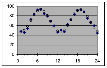
Example 4: Report and interpret the best-fit sinusoidal model for the dataset to the right, which records the amount that the average Fahrenheit temperature for a month is above or below the average temperature for the entire two-year period. The months are numbered starting with 1 for January 2003.

Solution approach:

[i] Copy the dataset to the Data Scratch Pad worksheet and display a scatter plot.

[ii] From the graph, make rough estimates of the amplitude and wavelength for the data, so that you will have values to use as initial parameter settings.

[iii] Use the model formula explained in this section to create a sinusoidal model worksheet from the General Model template in Models.xls, with parameters for wavelength, phase, and amplitude. Set the wavelength and amplitude parameters to the values you estimated in step [ii] above (leaving these parameters blank or zero will cause errors or confuse Solver).

[iv] Copy the dataset to the worksheet, then spread the formulas in columns C, D, and E down to match the data, as usual.

[v] Use Solver to find the best-fit parameters, and report your results.

Answer:

The best-fit sinusoidal model to this data has a wavelength of 11.9 months, a phase shift of 4.0 months, an amplitude of 23.3 degrees F, and a baseline average of 69.1 degrees F. The standard deviation for the fit is 2.8 degrees F.

Interpretation: The monthly temperature-difference averages at the location this data came from range by about 23 degrees above and below the yearly average of about 69 degrees. The pattern repeats about every 12 months, with the maximum-positive-slope point (i.e., spring) in April (month 4). Individual monthly averages can be expected to be within 2.8 degrees of this model about 2/3 of the time.

Month	Temp
1	47.8
2	45.3
3	54.0
4	72.6
5	83.4
6	91.9
7	92.9
8	84.8
9	79.5
10	69.1
11	60.1
12	46.4
13	50.8
14	47.4
15	62.8
16	71.9
17	83.1
18	91.2
19	93.4
20	88.4
21	75.5
22	67.0
23	59.6
24	44.3

The final worksheet should look similar to this:

x	y data	y model	Residual	Squared	y = $G$5 * SIN((x-$G$4)*6.2832/$G$3)
Input	Output	prediction	deviation	deviation	*Sinusoidal parameters*
1	47.8	46.37	1.43	2.0577	11.85328	Wavelength
2	45.3	49.43	-4.13	17.0726	3.960422	Phase shift
3	54	58.07	-4.07	16.5328	23.28311	Amplitude
4	72.6	69.89	2.71	7.3542
5	83.4	81.64	1.76	3.0990
6	91.9	90.08	1.82	3.3073	Model and data value counts
7	92.9	92.89	0.01	0.0002	3	Number of parameters
8	84.8	89.28	-4.48	20.0901	24	Number of dev. averaged
9	79.5	80.26	-0.76	0.5799
10	69.1	68.31	0.79	0.6226	Goodness of fit of this model
11	60.1	56.72	3.38	11.3938	169.8698	Sum of squared deviations
12	46.4	48.70	-2.30	5.2707	2.844124	Standard deviation
13	50.8	46.44	4.36	19.0293
14	47.4	50.57	-3.17	10.0663
15	62.8	59.96	2.84	8.0596
16	71.9	72.01	-0.11	0.0132
17	83.1	83.41	-0.31	0.0974
18	91.2	91.01	0.19	0.0357
19	93.4	92.72	0.68	0.4664
20	88.4	88.06	0.34	0.1155
21	75.5	78.32	-2.82	7.9745
22	67	66.19	0.81	0.6531
23	59.6	55.01	4.59	21.0864
24	44.3	47.85	-3.55	12.6379

$132.png$

Sinusoidal cycles and phases

Cycles: There is a close relationship between sinusoids and rotation. A spinning object repeats its sequence of positions every rotation, and the height of a point on a circle rotating at a constant speed varies over time according to a sinusoidal pattern. The wavelength of this sinusoid equals the rotation time of the circle, and the amplitude equals the radius of the circle. The phase is how long it has been since the point last passed the midpoint in an upward direction. The baseline is the height of the center of the circle.

Left-right shifts of the sinusoidal pattern: The standard sinusoid crosses the y axis where the curve has the steepest upward slope, where it is increasing past the average value. But the curve can be shifted right or left so that it crosses the y axis at some other point of the cycle. The distance from the nearest standard steepest-slope point to the actual crossing point is called the phase or the phase shift of the sinusoid. The phase shift is added to the x value before it is used inside the SIN function.

Two sinusoidal processes with the same wavelength can be in phase, in which case they will add together if they apply to the same measurement, or be out of phase, in which case there may be partial cancellation. Sometimes phase shifts are talked about in terms of angular degrees (e.g., “The electric and magnetic waves are 90 degrees out of phase”); this is based on taking a wavelength as being 360 degrees due to the analogy with rotation), so a phase shift of 90° means a phase shift of ¼ of the wavelength.

Mathematics for Modeling. Authored by: Mary Parker and Hunter Ellinger. License: CC BY: Attribution