
7.2: Evaluate and Graph Exponential Functions
- Page ID
- 29085

By the end of this section, you will be able to:
- Graph exponential functions
- Solve Exponential equations
- Use exponential models in applications
Before you get started, take this readiness quiz.
- Simplify: \(\left(\frac{x^{3}}{x^{2}}\right)\).
If you missed this problem, review Example 5.13. - Evaluate: a. \(2^{0}\) b. \(\left(\frac{1}{3}\right)^{0}\).
If you missed this problem, review Example 5.14. - Evaluate: a. \(2^{−1}\) b. \(\left(\frac{1}{3}\right)^{-1}\).
If you missed this problem, review Example 5.15.
Graph Exponential Functions
The functions we have studied so far do not give us a model for many naturally occurring phenomena. From the growth of populations and the spread of viruses to radioactive decay and compounding interest, the models are very different from what we have studied so far. These models involve exponential functions.
An exponential function is a function of the form \(f(x)=a^{x}\) where \(a>0\) and \(a≠1\).
An exponential function, where \(a>0\) and \(a≠1\), is a function of the form
\(f(x)=a^{x}\)
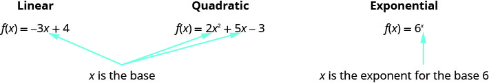
Notice that in this function, the variable is the exponent. In our functions so far, the variables were the base.
Our definition says \(a≠1\). If we let \(a=1\), then \(f(x)=a^{x}\) becomes \(f(x)=1^{x}\). Since \(1^{x}=1\) for all real numbers, \(f(x)=1\). This is the constant function.
Our definition also says \(a>0\). If we let a base be negative, say \(−4\), then \(f(x)=(−4)^{x}\) is not a real number when \(x=\frac{1}{2}\).
\(\begin{aligned} f(x) &=(-4)^{x} \\ f\left(\frac{1}{2}\right) &=(-4)^{\frac{1}{2}} \\ f\left(\frac{1}{2}\right) &=\sqrt{-4} \text { not a real number } \end{aligned}\)
In fact, \(f(x)=(−4)^{x}\) would not be a real number any time \(x\) is a fraction with an even denominator. So our definition requires \(a>0\).
By graphing a few exponential functions, we will be able to see their unique properties.
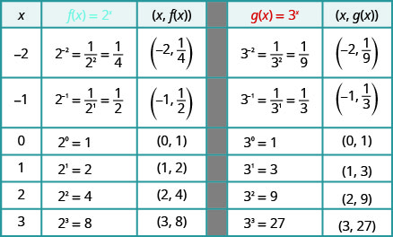
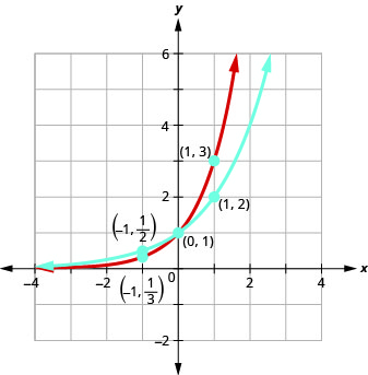
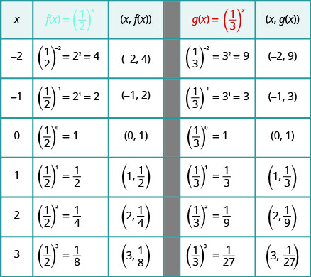
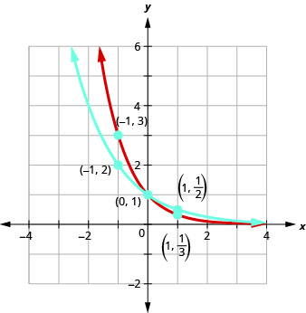
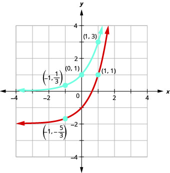
On the same coordinate system graph \(f(x)=2^{x}\) and \(g(x)=3^{x}\).
Solution:
We will use point plotting to graph the functions.
Graph: \(f(x)=4^{x}\).
- Answer
-
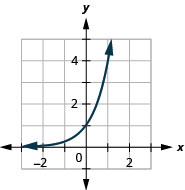
Figure 10.2.4
Graph: \(g(x)=5^{x}\)
- Answer
-
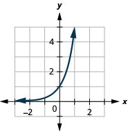
Figure 10.2.5
If we look at the graphs from the previous Example 10.2.1 and Exercises 10.2.1 and 10.2.2, we can identify some of the properties of exponential functions.
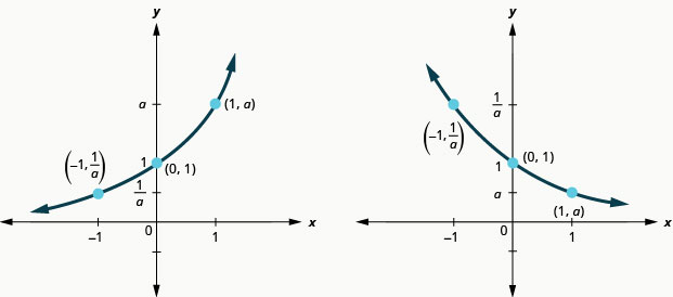
The graphs of \(f(x)=2^{x}\) and \(g(x)=3^{x}\), as well as the graphs of \(f(x)=4^{x}\) and \(g(x)=5^{x}\), all have the same basic shape. This is the shape we expect from an exponential function where \(a>1\).
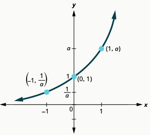
We notice, that for each function, the graph contains the point \((0,1)\). This make sense because \(a^{0}=1\) for any \(a\).
The graph of each function, \(f(x)=a^{x}\) also contains the point \((1,a)\). The graph of \(f(x)=2^{x}\) contained \((1,2)\) and the graph of \(g(x)=3^{x}\) contained \((1,3)\). This makes sense as \(a^{1}=a\).
Notice too, the graph of each function \(f(x)=a^{x}\) also contains the point \((−1,\frac{1}{a})\). The graph of \(f(x)=2^{x}\) contained \((−1,\frac{1}{2})\) and the graph of \(g(x)=3^{x}\) contained \((−1,\frac{1}{3})\).This makes sense as \(a^{−1}=\frac{1}{a}\).
What is the domain for each function? From the graphs we can see that the domain is the set of all real numbers. There is no restriction on the domain. We write the domain in interval notation as \((−∞,∞)\).
Look at each graph. What is the range of the function? The graph never hits the \(x\)-axis. The range is all positive numbers. We write the range in interval notation as \((0,∞)\).
Whenever a graph of a function approaches a line but never touches it, we call that line an asymptote. For the exponential functions we are looking at, the graph approaches the \(x\)-axis very closely but will never cross it, we call the line \(y=0\), the \(x\)-axis, a horizontal asymptote.
Properties of the Graph of \(f(x)=a^{x}\) when \(a>1\)
| Domain | \((-\infty, \infty)\) |
| Range | \((0, \infty)\) |
| \(x\)-intercept | None |
| \(y\)-intercept | \((0,1)\) |
| Contains | \((1, a),\left(-1, \frac{1}{a}\right)\) |
| Asymptote | \(x\)-axis, the line \(y=0\) |
Our definition of an exponential function \(f(x)=a^{x}\) says \(a>0\), but the examples and discussion so far has been about functions where \(a>1\). What happens when \(0<a<1\) The next example will explore this possibility.
On the same coordinate system, graph \(f(x)=\left(\frac{1}{2}\right)^{x}\) and \(g(x)=\left(\frac{1}{3}\right)^{x}\).
Solution:
We will use point plotting to graph the functions.
Graph: \(f(x)=\left(\frac{1}{4}\right)^{x}\).
- Answer
-
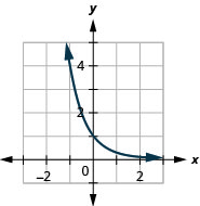
Figure 10.2.9
Graph: \(g(x)=\left(\frac{1}{5}\right)^{x}\).
- Answer
-
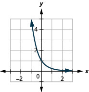
Figure 10.2.10
Now let’s look at the graphs from the previous Example 10.2.2 and Exercises 10.2.3 and 10.2.4 so we can now identify some of the properties of exponential functions where \(0<a<1\).
The graphs of \(f(x)=\left(\frac{1}{2}\right)^{x}\) and \(g(x)=\left(\frac{1}{3}\right)^{x}\) as well as the graphs of \(f(x)=\left(\frac{1}{4}\right)^{x}\) and \(g(x)=\left(\frac{1}{5}\right)^{x}\) all have the same basic shape. While this is the shape we expect from an exponential function where \(0<a<1\), the graphs go down from left to right while the previous graphs, when \(a>1\), went from up from left to right.
We notice that for each function, the graph still contains the point \((0, 1)\). This make sense because \(a^{0}=1\) for any \(a\).
As before, the graph of each function, \(f(x)=a^{x}\), also contains the point \((1,a)\). The graph of \(f(x)=\left(\frac{1}{2}\right)^{x}\) contained \(\left(1, \frac{1}{2}\right)\) and the graph of \(g(x)=\left(\frac{1}{3}\right)^{x}\) contained \(\left(1, \frac{1}{3}\right)\). This makes sense as \(a^{1}=a\).
Notice too that the graph of each function, \(f(x)=a^{x}\), also contains the point \(\left(-1, \frac{1}{a}\right)\). The graph of \(f(x)=\left(\frac{1}{2}\right)^{x}\) contained \((−1,2)\) and the graph of \(g(x)=\left(\frac{1}{3}\right)^{x}\) contained \((−1,3)\). This makes sense as \(a^{-1}=\frac{1}{a}\).
What is the domain and range for each function? From the graphs we can see that the domain is the set of all real numbers and we write the domain in interval notation as \((−∞,∞)\). Again, the graph never hits the \(x\)-axis. The range is all positive numbers. We write the range in interval notation as \((0,∞)\).
We will summarize these properties in the chart below. Which also include when \(a>1\).
Properties of the Graph of \(f(x)=a^{x}\)
| When \(a>1\) | When \(0<a<1\) | ||
|---|---|---|---|
| 1\)">Domain | \((-\infty, \infty)\) | Domain | \((-\infty, \infty)\) |
| 1\)">Range | \((0, \infty)\) | Range | \((0, \infty)\) |
| 1\)">\(x\)-intercept | none | \(x\)-intercept | none |
| 1\)">\(y\)-intercept | \((0,1)\) | \(y\)-intercept | \((0,1)\) |
| 1\)">Contains | \((1, a),\left(-1, \frac{1}{a}\right)\) | Contains | \((1, a),\left(-1, \frac{1}{a}\right)\) |
| 1\)">Asymptote |
\(x\)-axis, the line \(y=0\) |
Asymptote | \(x\)-axis, the line \(y=0\) |
| 1\)">Basic Shape | increasing | Basic Shape | decreasing |
It is important for us to notice that both of these graphs are one-to-one, as they both pass the horizontal line test. This means the exponential function will have an inverse. We will look at this later.
When we graphed quadratic functions, we were able to graph using translation rather than just plotting points. Will that work in graphing exponential functions?
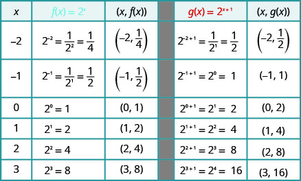
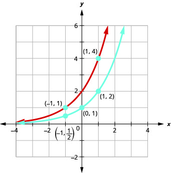
On the same coordinate system graph \(f(x)=2^{x}\) and \(g(x)=2^{x+1}\).
Solution:
We will use point plotting to graph the functions.
On the same coordinate system, graph: \(f(x)=2^{x}\) and \(g(x)=2^{x-1}\).
- Answer
-
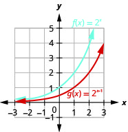
Figure 10.2.14
On the same coordinate system, graph \(f(x)=3^{x}\) and \(g(x)=3^{x+1}\).
- Answer
-
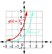
Figure 10.2.15
Looking at the graphs of the functions \(f(x)=2^{x}\) and \(g(x)=2^{x+1}\) in the last example, we see that adding one in the exponent caused a horizontal shift of one unit to the left. Recognizing this pattern allows us to graph other functions with the same pattern by translation.
Let’s now consider another situation that might be graphed more easily by translation, once we recognize the pattern.
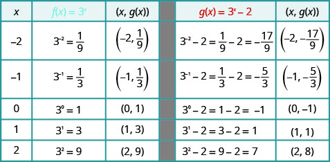
On the same coordinate system graph \(f(x)=3^{x}\) and \(g(x)=3^{x}-2\).
Solution:
We will use point plotting to graph the functions.
On the same coordinate system, graph \(f(x)=3^{x}\) and \(g(x)=3^{x}+2\).
- Answer
-
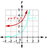
Figure 10.2.18
On the same coordinate system, graph \(f(x)=4^{x}\) and \(g(x)=4^{x}-2\).
- Answer
-
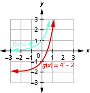
Figure 10.2.19
Looking at the graphs of the functions \(f(x)=3^{x}\) and \(g(x)=3^{x}−2\) in the last example, we see that subtracting \(2\) caused a vertical shift of down two units. Notice that the horizontal asymptote also shifted down \(2\) units. Recognizing this pattern allows us to graph other functions with the same pattern by translation.
All of our exponential functions have had either an integer or a rational number as the base. We will now look at an exponential function with an irrational number as the base.
Before we can look at this exponential function, we need to define the irrational number, \(e\). This number is used as a base in many applications in the sciences and business that are modeled by exponential functions. The number is defined as the value of \(\left(1+\frac{1}{n}\right)^{n}\) as \(n\) gets larger and larger. We say, as \(n\) approaches infinity, or increases without bound. The table shows the value of \(\left(1+\frac{1}{n}\right)^{n}\) for several values of \(n\).
| \(n\) | \(\left(1+\frac{1}{n}\right)^{n}\) |
|---|---|
| \(1\) | \(2\) |
| \(2\) | \(2.25\) |
| \(5\) | \(2.48832\) |
| \(10\) | \(2.59374246\) |
| \(100\) | \(2.704813829 \ldots\) |
| \(1,000\) | \(2.716923932 \ldots\) |
| \(10,000\) | \(2.718145927 \ldots\) |
| \(100,000\) | \(2.718268237 \ldots\) |
| \(1,000,000\) | \(2.718280469 \ldots\) |
| \(1,000,000,000\) | \(2.718281827 \ldots\) |
\(e \approx 2.718281827\)
The number \(e\) is like the number \(π\) in that we use a symbol to represent it because its decimal representation never stops or repeats. The irrational number \(e\) is called the natural base.
Natural Base \(e\)
The number \(e\) is defined as the value of \(\left(1+\frac{1}{n}\right)^{n}\), as \(n\) increases without bound. We say, as \(n\) approaches infinity,
\(e \approx 2.718281827\)
The exponential function whose base is \(e\), \(f(x)=e^{x}\) is called the natural exponential function.
Natural Exponential Function
The natural exponential function is an exponential function whose base is \(e\)
\(f(x)=e^{x}\)
The domain is \((−∞,∞)\) and the range is \((0,∞)\).
Let’s graph the function \(f(x)=e^{x}\) on the same coordinate system as \(g(x)=2^{x}\) and \(h(x)=3^{x}\).
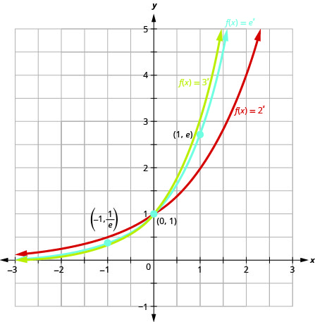
Notice that the graph of \(f(x)=e^{x}\) is “between” the graphs of \(g(x)=2^{x}\) and \(h(x)=3^{x}\).Does this make sense as \(2<e<3\)?
Solve Exponential Equations
Equations that include an exponential expression \(a^{x}\) are called exponential equations. To solve them we use a property that says as long as \(a>0\) and \(a≠1\), if \(a^{x}=a^{y}\) then it is true that \(x=y\). In other words, in an exponential equation, if the bases are equal then the exponents are equal.
One-to-One Property of Exponential Equations
For \(a>0\) and \(a≠1\),
If \(a^{x}=a^{y}\),then \(x=y\).
To use this property, we must be certain that both sides of the equation are written with the same base.
Solve: \(3^{2 x-5}=27\).
Solution:
| Step 1: Write both sides of the equation with the same base. | Since the left side has base \(3\), we write the right side with base \(3\). \(27=3^{3}\) | \(3^{2 x-5}=27\) \(3^{2 x-5}=3^{3}\) |
| Step 2: Write a new equation by setting the exponents equal. | Since the bases are the same, the exponents must be equal. | \(2x-5=3\) |
| Step 3: Solve the equation. |
Add \(5\) to each side. Divide by \(2\). |
\(\begin{aligned} 2 x &=8 \\ x &=4 \end{aligned}\) |
| Step 4: Check the solution. | Substitute \(x=4\) into the original equation. | \(\begin{aligned} 3^{2 x-5} &=27 \\ 3^{2 \cdot \color{red}{4}\color{black}{-}5} & \stackrel{?}{=} 27 \\ 3^{3} &\stackrel{?}{=}27 \\ 27 &=27 \end{aligned}\) |
Solve: \(3^{3 x-2}=81\).
- Answer
-
\(x=2\)
Solve: \(7^{x-3}=7\).
- Answer
-
\(x=4\)
The steps are summarized below.
How to Solve an Exponential Function
- Write both sides of the equation with the same base, if possible.
- Write a new equation by setting the exponents equal.
- Solve the equation.
- Check the solution.
In the next example, we will use our properties on exponents.
Solve \(\frac{e^{x^{2}}}{e^{3}}=e^{2 x}\).
Solution:
| \(\frac{e^{x^{2}}}{e^{3}}=e^{2 x}\) | |
| Use the Property of Exponents: \(\frac{a^{m}}{a^{n}}=a^{m-n}\). | \(e^{x^{2}-3}=e^{2 x}\) |
| Write a new equation by setting the exponents equal. | \(x^{2}-3=2 x\) |
| Solve the equation. | \(x^{2}-2 x-3=0\) |
| \((x-3)(x+1)=0\) | |
| \(x=3, x=-1\) | |
| Check the solutions. | |
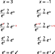 |
Solve: \(\frac{e^{x^{2}}}{e^{x}}=e^{2}\).
- Answer
-
\(x=-1, x=2\)
Solve: \(\frac{e^{x^{2}}}{e^{x}}=e^{6}\).
- Answer
-
\(x=-2, x=3\)
Use Exponential Models in Applications
Exponential functions model many situations. If you own a bank account, you have experienced the use of an exponential function. There are two formulas that are used to determine the balance in the account when interest is earned. If a principal, \(P\), is invested at an interest rate, \(r\), for \(t\) years, the new balance, \(A\), will depend on how often the interest is compounded. If the interest is compounded \(n\) times a year we use the formula \(A=P\left(1+\frac{r}{n}\right)^{n t}\). If the interest is compounded continuously, we use the formula \(A=Pe^{rt}\). These are the formulas for compound interest.
Compound Interest
For a principal, \(P\), invested at an interest rate, \(r\), for \(t\) years, the new balance, \(A\), is:
\(\begin{array}{ll}{A=P\left(1+\frac{r}{n}\right)^{n t}} & {\text { when compounded } n \text { times a year. }} \\ {A=P e^{r t}} & {\text { when compounded continuously. }}\end{array}\)
As you work with the Interest formulas, it is often helpful to identify the values of the variables first and then substitute them into the formula.
A total of $\(10,000\) was invested in a college fund for a new grandchild. If the interest rate is \(5\)%, how much will be in the account in \(18\) years by each method of compounding?
- compound quarterly
- compound monthly
- compound continuously
Solution:
Identify the values of each variable in the formulas. Remember to express the percent as a decimal.
\(\begin{aligned} A &=? \\ P &=\$ 10,000 \\ r &=0.05 \\ t &=18 \text { years } \end{aligned}\)
a. For quarterly compounding, \(n=4\). There are \(4\) quarters in a year.
\(A=P\left(1+\frac{r}{n}\right)^{n t}\)
Substitute the values in the formula.
\(A=10,000\left(1+\frac{0.05}{4}\right)^{4 \cdot 18}\)
Compute the amount. Be careful to consider the order of operations as you enter the expression into your calculator.
\(A=\$ 24,459.20\)
b. For monthly compounding, \(n=12\).There are \(12\) months in a year.
\(A=P\left(1+\frac{r}{n}\right)^{n t}\)
Substitute the values in the formula.
\(A=10,000\left(1+\frac{0.05}{12}\right)^{12 \cdot 18}\)
Compute the amount.
\(A=\$ 24,550.08\)
c. For compounding continuously,
\(A=P e^{r t}\)
Substitute the values in the formula.
\(A=10,000 e^{0.05 \cdot 18}\)
Compute the amount.
\(A=\$ 24,596.03\)
Angela invested $\(15,000\) in a savings account. If the interest rate is \(4\)%, how much will be in the account in \(10\) years by each method of compounding?
- compound quarterly
- compound monthly
- compound continuously
- Answer
-
- $\(22,332.96\)
- $\(22,362.49\)
- $\(22,377.37\)
Allan invested $\(10,000\) in a mutual fund. If the interest rate is \(5\)%, how much will be in the account in \(15\) years by each method of compounding?
- compound quarterly
- compound monthly
- compound continuously
- Answer
-
- $\(21,071.81\)
- $\(21,137.04\)
- $\(21,170.00\)
Other topics that are modeled by exponential functions involve growth and decay. Both also use the formula \(A=Pe^{rt}\) we used for the growth of money. For growth and decay, generally we use \(A_{0}\), as the original amount instead of calling it \(P\), the principal. We see that exponential growth has a positive rate of growth and exponential decay has a negative rate of growth.
Exponential Growth and Decay
For an original amount, \(A_{0}\), that grows or decays at a rate, \(r\), for a certain time, \(t\), the final amount, \(A\), is:
\(A=A_{0} e^{r t}\)
Exponential growth is typically seen in the growth of populations of humans or animals or bacteria. Our next example looks at the growth of a virus.
Chris is a researcher at the Center for Disease Control and Prevention and he is trying to understand the behavior of a new and dangerous virus. He starts his experiment with \(100\) of the virus that grows at a rate of \(25\)% per hour. He will check on the virus in \(24\) hours. How many viruses will he find?
Solution:
Identify the values of each variable in the formulas. Be sure to put the percent in decimal form. Be sure the units match--the rate is per hour and the time is in hours.
\(\begin{aligned} A &=? \\ A_{0} &=100 \\ r &=0.25 / \text { hour } \\ t &=24 \text { hours } \end{aligned}\)
Substitute the values in the formula: \(A=A_{0} e^{r t}\).
\(A=100 e^{0.25 \cdot 24}\)
Compute the amount.
\(A=40,342.88\)
Round to the nearest whole virus.
\(A=40,343\)
The researcher will find \(40,343\) viruses.
Another researcher at the Center for Disease Control and Prevention, Lisa, is studying the growth of a bacteria. She starts his experiment with \(50\) of the bacteria that grows at a rate of \(15\)% per hour. He will check on the bacteria every \(8\) hours. How many bacteria will he find in \(8\) hours?
- Answer
-
She will find \(166\) bacteria.
Maria, a biologist is observing the growth pattern of a virus. She starts with \(100\) of the virus that grows at a rate of \(10\)% per hour. She will check on the virus in \(24\) hours. How many viruses will she find?
- Answer
-
She will find \(1,102\) viruses.
Access these online resources for additional instruction and practice with evaluating and graphing exponential functions.
Key Concepts
- Properties of the Graph of \(f(x)=a^{x}\):
| When \(a>1\) | When \(0<a<1\) | ||
|---|---|---|---|
| 1\)">Domain | \((-\infty, \infty)\) | Domain | \((-\infty, \infty)\) |
| 1\)">Range | \((0, \infty)\) | Range | \((0, \infty)\) |
| 1\)">\(x\)-intercept | none | \(x\)-intercept | none |
| 1\)">\(y\)-intercept | \((0,1)\) | \(y\)-intercept | \((0,1)\) |
| 1\)">Contains | \((1, a),\left(-1, \frac{1}{a}\right)\) | Contains | \((1, a),\left(-1, \frac{1}{a}\right)\) |
| 1\)">Asymptote |
\(x\)-axis, the line \(y=0\) |
Asymptote | \(x\)-axis, the line \(y=0\) |
| 1\)">Basic Shape | increasing | Basic Shape | decreasing |
- One-to-One Property of Exponential Equations:
For \(a>0\) and \(a≠1\),\(A=A_{0} e^{r t}\)
- How to Solve an Exponential Equation
- Write both sides of the equation with the same base, if possible.
- Write a new equation by setting the exponents equal.
- Solve the equation.
- Check the solution.
- Compound Interest: For a principal, \(P\), invested at an interest rate, \(r\), for \(t\) years, the new balance, \(A\), is
\(\begin{array}{ll}{A=P\left(1+\frac{r}{n}\right)^{n t}} & {\text { when compounded } n \text { times a year. }} \\ {A=P e^{r t}} & {\text { when compounded continuously. }}\end{array}\) - Exponential Growth and Decay: For an original amount, \(A_{0}\) that grows or decays at a rate, \(r\), for a certain time \(t\), the final amount, \(A\), is \(A=A_{0}e^{rt}\).
Glossary
- asymptote
- A line which a graph of a function approaches closely but never touches.
- exponential function
- An exponential function, where \(a>0\) and \(a≠1\), is a function of the form \(f(x)=a^{x}\).
- natural base
- The number \(e\) is defined as the value of \((1+\frac{1}{n})^{n}\), as \(n\) gets larger and larger. We say, as \(n\) increases without bound, \(e≈2.718281827...\)
- natural exponential function
- The natural exponential function is an exponential function whose base is \(e\): \(f(x)=e^{x}\). The domain is \((−∞,∞)\) and the range is \((0,∞)\).