3.6: Zeros of Polynomial Functions

Last updated
Save as PDF

Page ID: 34894

$ \newcommand{\vecs}[1]{\overset { \scriptstyle \rightharpoonup} {\mathbf{#1}} } $ $ \newcommand{\vecd}[1]{\overset{-\!-\!\rightharpoonup}{\vphantom{a}\smash {#1}}} $$\newcommand{\id}{\mathrm{id}}$ $ \newcommand{\Span}{\mathrm{span}}$ $ \newcommand{\kernel}{\mathrm{null}\,}$ $ \newcommand{\range}{\mathrm{range}\,}$ $ \newcommand{\RealPart}{\mathrm{Re}}$ $ \newcommand{\ImaginaryPart}{\mathrm{Im}}$ $ \newcommand{\Argument}{\mathrm{Arg}}$ $ \newcommand{\norm}[1]{\| #1 \|}$ $ \newcommand{\inner}[2]{\langle #1, #2 \rangle}$ $ \newcommand{\Span}{\mathrm{span}}$ $\newcommand{\id}{\mathrm{id}}$ $ \newcommand{\Span}{\mathrm{span}}$ $ \newcommand{\kernel}{\mathrm{null}\,}$ $ \newcommand{\range}{\mathrm{range}\,}$ $ \newcommand{\RealPart}{\mathrm{Re}}$ $ \newcommand{\ImaginaryPart}{\mathrm{Im}}$ $ \newcommand{\Argument}{\mathrm{Arg}}$ $ \newcommand{\norm}[1]{\| #1 \|}$ $ \newcommand{\inner}[2]{\langle #1, #2 \rangle}$ $ \newcommand{\Span}{\mathrm{span}}$$\newcommand{\AA}{\unicode[.8,0]{x212B}}$

Learning Objectives

Evaluate a polynomial using the Remainder Theorem.
Use the Factor Theorem to solve a polynomial equation.
Use the Rational Zero Theorem to find rational zeros.
Find zeros of a polynomial function.
Theorems to simplify search for zeros: Lower & Upper Bound Theorem, Intermediate Value Theorem, Descartes' Rule of Signs
Use the Linear Factorization Theorem to find polynomials with given zeros.

In this section, we will discuss a variety of tools for writing polynomial functions and solving polynomial equations.

Evaluate a Polynomial Using the Remainder Theorem

In the last section, we learned how to divide polynomials. We can now use polynomial division to evaluate polynomials using the Remainder Theorem. If the polynomial is divided by $x–k$, the remainder may be found quickly by evaluating the polynomial function at $k$, that is, $f(k)$. Let’s walk through the proof of the theorem.

Recall that the Division Algorithm states that, given a polynomial dividend $f(x)$ and a non-zero polynomial divisor $d(x)$ where the degree of $d(x)$ is less than or equal to the degree of $f(x)$, there exist unique polynomials $q(x)$ and $r(x)$ such that $f(x)=d(x)q(x)+r(x) $.

If the divisor, $d(x)$, is $x−k$, this takes the form $f(x)=(x−k)q(x)+r $. Since the divisor $x−k$ is linear, the remainder will be a constant, $r$. And, if we evaluate $f(x)$ for $x=k$, we have

\[\begin{align*} f(k)&=(k−k)q(k)+r \\[4pt] &=0{\cdot}q(k)+r \&=r \end{align*}\]

In other words, $f(k)$ is the remainder obtained by dividing $f(x)$ by $x−k$.

The Remainder Theorem

If a polynomial $f(x)$ is divided by $x−k$, then the remainder is the value $f(k)$.

$how-to.png$ How to: Use the Remainder Theorem to evaluate $f(x)$ at $x=k$.

Use synthetic division to divide the polynomial by $x−k$.
The remainder is the value $f(k)$.

Example $\PageIndex{1}$: Use the Remainder Theorem to Evaluate a Polynomial

Use the Remainder Theorem to evaluate $f(x)=6x^4−x^3−15x^2+2x−7$ at $x=2$.

Solution

To find the remainder using the Remainder Theorem, use synthetic division to divide the polynomial by $x−2$.

$
{\begin{array}{c}
2\\ \\ \\ \end{array}}{\begin{align*}&\\[0pt]&{\begin{array}{r|}\\[0pt] \\[0pt] \end{array}}\\[1pt]& \\[2pt]& \end{align*}}\!\!
{\begin{array}{rrrr}
6 & −1 & −15 & 2 & −7\\
& 12 & 22 & 14 & 32 \\
\hline 6 & 11 & 7 & 16 & 25
\end{array}}
$

The remainder is 25. Therefore, $f(2)=25$.

Analysis

We can check our answer by evaluating $f(2)$.

\[\begin{align*} f(x)&=6x^4−x^3−15x^2+2x−7 \\ f(2)&=6(2)^4−(2)^3−15(2)^2+2(2)−7=25 \end{align*}\]

$try-it.png$ Try It $\PageIndex{1}$

Use the Remainder Theorem to evaluate $f(x)=2x^5−3x^4−9x^3+8x^2+2$ at $x=−3$.

Answer: $f(−3)=−412$

Use the Factor Theorem to Solve a Polynomial Equation

The Factor Theorem is another theorem that helps us analyze polynomial equations. It tells us how the zeros of a polynomial are related to the factors. Recall the definition of a zero, $k,$ of $f,$ is $f(k)=0$ and that the Division Algorithm states

\[f(x)=(x−k)q(x)+r \nonumber\]

If $k$ is a zero of $f(x)$, then $f(k)=0$. Therefore $f(k)=(k-k)q(k)+r = 0$ and thus $r=0$. Because the remainder $r$ of $f(k)$ is $0,$ then $f (x)=(x−k)q(x)+0$ or $f(x)=(x−k)q(x)$. Notice, written in this form, $x−k$ is a factor of $f(x)$. We can conclude if $k$ is a zero of $f(x)$, then $x−k$ is a factor of $f(x)$.

Conversely, if $x−k$ is a factor of $f(x)$, then the remainder $r$ of the Division Algorithm $f(x)=(x−k)q(x)+r$ is $0$. Therefore $f(x)=(x−k)q(x)+r = (x−k)q(x)+0=(x-k)q(x).$ Evaluating $f$ when $x=k$ we obtain $f(k)= 0$. Since $f(k)=0$ we can conclude $k$ is a zero of $f(x)$.

This pair of implications is the Factor Theorem. As we will soon see, a polynomial of degree $n$ in the complex number system will have $n$ zeros. We can use the Factor Theorem to completely factor a polynomial into the product of $n$ factors. Once the polynomial has been completely factored, we can easily determine the zeros of the polynomial.

THE FACTOR THEOREM

According to the Factor Theorem, $k$ is a zero of $f(x)$ if and only if $(x−k)$ is a factor of $f(x)$.

$how-to.png$ How to: Factor a third-degree polynomial, given one of its factors.

Use synthetic division to divide the polynomial by $(x−k)$.
Confirm that the remainder is $0$.
Write the polynomial as the product of $(x−k)$ and the quadratic quotient.
If possible, factor the quadratic and write the polynomial as the product of three linear factors.
Otherwise, write it as the product of a linear factor and an irreducible quadratic factor.

Example $\PageIndex{2}$: Use the Factor Theorem to Solve a Polynomial Equation

Show that $(x+2)$ is a factor of $x^3−6x^2−x+30$. Find the remaining factors. Use the factors to determine the zeros of the polynomial.

Solution

We can use synthetic division to show that $(x+2)$ is a factor of the polynomial.

$
{\begin{array}{c}
-2\\ \\ \\ \end{array}}{\begin{align*}&\\[0pt]&{\begin{array}{r|}\\[0pt] \\[0pt] \end{array}}\\[1pt]& \\[2pt]& \end{align*}}\!\!
{\begin{array}{rrrr}
1 & −6 & −1 & 30\\
& -2 & 16 & -30 \\
\hline 1 & -8 & 15 & 0
\end{array}}
$

The remainder is zero, so $(x+2)$ is a factor of the polynomial. We can use the Division Algorithm to write the polynomial as the product of the divisor and the quotient:

$x^3−6x^2−x+30 = (x+2)(x^2−8x+15)$

We can factor the quadratic factor to write the polynomial as a product of linear factors

$x^3−6x^2−x+30 = (x+2)(x−3)(x−5)$

By the Factor Theorem, the zeros of $x^3−6x^2−x+30$ are –2, 3, and 5.

$try-it.png$ Try It $\PageIndex{2}$

Use the Factor Theorem to find the zeros of $f(x)=x^3+4x^2−4x−16$ given that $(x−2)$ is a factor of the polynomial.

Answer: The zeros are 2, –2, and –4.

Use the Rational Zero Theorem to Find Rational Zeros

Another use for the Remainder Theorem is to test whether a rational number is a zero for a given polynomial. But first we need a pool of rational numbers to test. The Rational Zero Theorem helps us to narrow down the number of possible rational zeros using the ratio of the factors of the constant term and the factors of the leading coefficient of the polynomial

Consider a quadratic function with two zeros $x=\dfrac{ {\color{red}{2}} }{ {\color{Cerulean}{5}} }$ and $x=\dfrac{ {\color{red}{3}} }{ {\color{Cerulean}{4}} }$. By the Factor Theorem, these zeros have factors associated with them. Let us set each factor equal to 0, and then construct the original quadratic function.

$CNX_Precalc_Figure_03_03_022.jpg$

Notice that two factors of the constant term, 6, are the two numerators from the original rational roots: ${\color{red}{2}}$ and ${\color{red}{3}}$. Similarly, two of the factors from the leading coefficient, 20, are the two denominators from the original rational roots: ${\color{Cerulean}{5}}$ and ${\color{Cerulean}{4}}$.

We can infer that the numerators of the rational roots will always be factors of the constant term and the denominators will be factors of the leading coefficient. This is the essence of the Rational Zero Theorem; it is a means to give us a pool of possible rational zeros.

THE RATIONAL ZERO THEOREM

If the polynomial $f(x)={\color{Cerulean}{a_n}}x^n+a_{n−1}x^{n−1}+...+a_1x+{\color{red}{a_0}}$ has integer coefficients, then every rational zero of $f(x)$ has the form $ \dfrac{ {\color{red}{p}} }{ {\color{Cerulean}{q}} }$ where $p$ is a factor of the constant term $a_0$ and $q$ is a factor of the leading coefficient $a_n$.

When the leading coefficient is 1, the possible rational zeros are the factors of the constant term.

$how-to.png$ How to: Use the Rational Zero Theorem to find all a polynomial's rational zeros.

Determine all factors of the constant term and all factors of the leading coefficient.
Determine all possible values of $\dfrac{ {\color{red}{p}} }{ {\color{Cerulean}{q}} }$ , where $p$ is a factor of the constant term and $q$ is a factor of the leading coefficient. Be sure to include both positive and negative candidates.
Determine which possible zeros are actual zeros by using synthetic division. If the remainder is zero, a zero has been found. If the zero found is $z$, then $f$ can be rewritten as a product of $ (x-z) $ and a quotient. The quotient is a polynomial that is one degree less than $f$.
Repeat the search for zeros, but this time search for a zero of the quotient rather than $f$. The search for zeros is repeated until the quotient obtained is a quadratic or linear factor. When searching for zeros, remember that the same value for a zero can occur more than once, and that if a value is found to not be a zero for one quotient, it will not be a zero for any of the quotients.

Example $\PageIndex{3}$: List All Possible Rational Zeros

List all possible rational zeros of $f(x)=2x^4−5x^3+x^2−4$.

Solution:

The only possible rational zeros of $f(x)$ are quotients of factors of the constant term, –4, and the leading coefficient, 2.

The constant term is –4; the factors of –4 are $p=±1,±2,±4$.

The leading coefficient is 2; the factors of 2 are $q=±1,±2$.

If any of the four real zeros are rational zeros, then they will be of one of the following factors of –4 divided by one of the factors of 2.

\[\dfrac{p}{q}=±\dfrac{1}{1},±\dfrac{2}{1},±\dfrac{4}{1} \; \; \; \; \; \; \frac{p}{q}=±\dfrac{1}{2},±\dfrac{2}{2},±\dfrac{4}{2} \nonumber\]

Note that $\frac{2}{2}=1$ and $\frac{4}{2}=2$, which have already been listed. So we can shorten our list.

\[\dfrac{p}{q} = \dfrac{\text{Factors of the constant term}}{\text{Factors of the leading coefficient}}=±1,±2,±4,±\dfrac{1}{2}\nonumber \]

Example $\PageIndex{4}$: Use the Rational Zero Theorem to Find Rational Zeros

Use the Rational Zero Theorem to find the rational zeros of $f(x)=2x^3+x^2−4x+1$.

Solution. The Rational Zero Theorem tells us that all possible rational zeros have the form $\frac{p}{q}$ where $p$ is a factor of 1 and $q$ is a factor of 2.

\[ \begin{align*} \dfrac{p}{q}=\dfrac{\text{factor of constant term}}{\text{factor of coefficient}} &=\dfrac{\text{factor of }1}{\text{factor of }2} \end{align*}\]

The factors of 1 are ±1 and the factors of 2 are ±1 and ±2. The possible values for $\frac{p}{q}$ are ±1 and $±\frac{1}{2}$. These are the possible rational zeros for the function. We can determine which of the possible zeros are actual zeros by using synthetic division and trying each of these values as the divisor.

$
{\begin{array}{c}
1\\ \\ \\ \end{array}}{\begin{align*}&\\[0pt]&{\begin{array}{r|}\\[0pt] \\[0pt] \end{array}}\\[1pt]& \\[2pt]& \end{align*}}\!\!
{\begin{array}{rrrr}
2 & 1 & −4 & 1\\
& 2 & 3 & -1 \\
\hline 2 & 3 & -1 & 0
\end{array}}
$

The remainder is zero, so $f(x)$ can be factored as $f(x)=(x-1)(2x^2+3x-1)$. The zeros of the quadratic expression can be found by using the quadratic formula. The zeros are $ \frac{-3 \pm \sqrt{17}}{4} $, which are irrational numbers, so the only rational zero of $f$ is $1$.

$try-it.png$ Try It $\PageIndex{4}$

Use the Rational Zero Theorem to find the rational zeros of $f(x)=x^3−5x^2+2x+1$.

Answer: There are no rational zeros. All the zeros are irrational numbers or imaginary numbers rather than rational numbers.

Find all the Zeros of a Polynomial Function

The Rational Zero Theorem helps us to narrow down the list of possible rational zeros for a polynomial function. Once we have done this, we can use synthetic division repeatedly to determine all of the zeros of a polynomial function.

$how-to.png$ How to: Use synthetic division to find a polynomial's zeroes.

Use the Rational Zero Theorem to list all possible rational zeros of the function $f$.
Go through the list of possible rational zeros by performing synthetic division on $ \dfrac {f(x)}{x-c} $, where $c$ is in the list of possible rational zeros. When the remainder is 0, then a zero has been found: $c$.
Rewrite $f$ as a product of $x-c$ and a quotient. (The quotient will always be one degree less than $f$). Repeat steps 1 and 2 on the quotient (rather than on $f$ ) until the new quotient is a quadratic.
Find the zeros of the quadratic function. Two possible methods for solving quadratics are factoring and using the quadratic formula.

Example $\PageIndex{5}$: Find the Zeros of a Polynomial Function with Repeated Real Zeros

Find the zeros of $f(x)=4x^3−3x−1$.

Solution:

Step 1. The Rational zeros are $±1$,$±\dfrac{1}{2}$, and $±\dfrac{1}{4}$ because by the Rational Zero Theorem, if $\dfrac{p}{q}$ is a zero of $f(x)$, then

\[ \begin{align*} \dfrac{p}{q}=\dfrac{\text{factor of constant term}}{\text{factor of coefficient}} &=\dfrac{\text{factor of }-1}{\text{factor of }4} &=\dfrac{±1}{±1,±2, or ±4}\end{align*}\]

Step 2. Use synthetic division to test each possible zero until we find one that gives a remainder of 0. Let’s begin with 1.

$xCNX_CAT_Figure_05_01_012.jpg$

Step 3. Dividing by $(x−1)$ gives a remainder of 0, so 1 is a zero of the function. The polynomial can be written as $(x−1)(4x^2+4x+1) $

Step 4. The quotient is a quadratic. The quadratic can be factored. It is a perfect square. $f(x)$ can be written as $ f(x)=(x−1)(2x+1)^2 $. We already know that 1 is a zero. The other zero will have a multiplicity of 2 because the factor is squared. To find the other zero, we can set the factor equal to 0.

$ 2x+1=0 \qquad \longrightarrow \qquad x =−\dfrac{1}{2} $

$CNX_Precalc_Figure_03_06_001.jpg$ The zeros of the function are 1 with odd multiplicity of 1 and $−\frac{1}{2}$ with even multiplicity of 2.

Analysis

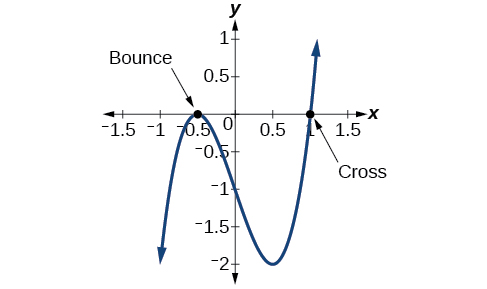
Look at the graph of the function $f$ shown on the right.

Notice, at $x =−0.5$, the graph bounces off the x-axis, indicating the even multiplicity $(2,\;4,\;6…)$ for the zero −0.5.

At $x=1$, the graph crosses the x-axis, indicating the odd multiplicity $(1,\;3,\;5…)$ for the zero $x=1$

Example $\PageIndex{6}$: Find zeros of a degree 4 polynomial

Find the zeros of $f(x) = x^4+2x^3-3x^2-4x+4$.

Solution

Step 1. Possible rational zeros of $f$ are $ \pm 1 \, \pm \, 2\, \pm \, 4 $

Step 2. Use synthetic division with each candidate in this list until a remainder of zero is found. Below shows that a zero $ x = 1 $ has been found.

$
{\begin{array}{c}
1\\ \\ \\ \end{array}}{\begin{align*}&\\[0pt]&{\begin{array}{r|}\\[0pt] \\[0pt] \end{array}}\\[1pt]& \\[2pt]& \end{align*}}\!\!
{\begin{array}{rrrr}
1 & 2 & −3 & -4 & 4\\
& 1 & 3 & 0 & -4 \\
\hline 1 & 3 & 0 & -4 & 0
\end{array}}
$

Step 3. $f(x) = (x-1)(Q(x)) $. The quotient polynomial, $Q(x) = x^3 + 3x^2 -4 $, is a third degree polynomial, so another round of searching for a zero needs to be done, this time on the quotient, $Q(x) = x^3 + 3x^2 -4 $

Step 1. Possible rational zeros of $Q$ are (still) $ \pm \, 1, \pm \, 2\, \pm \, 4 $

Step 2. Use synthetic division with each candidate in this list until a remainder of zero is found. It doesn't hurt to try $1$ again. Below shows that another zero $ x = 1 $ has been found.

$
{\begin{array}{c}
1\\ \\ \\ \end{array}}{\begin{align*}&\\[0pt]&{\begin{array}{r|}\\[0pt] \\[0pt] \end{array}}\\[1pt]& \\[2pt]& \end{align*}}\!\!
{\begin{array}{rrrr}
1 & 3 & 0 & −4\\
& 1 & 4 & 4 \\
\hline 1 & 4 & 4 & 0
\end{array}}
$

Step 3. $Q(x) = (x+1)( R(x) )$, so $f(x) = (x-1)(Q(x)) \longrightarrow f(x) = (x-1)(x-1)(R(x)).$ The quotient polynomial, $ R(x) = x^2 +4x+4,$ is a quadratic.

Step 4. Setting this quadratic to zero gives $x^2 +4x+4= 0$, or $ (x+2)(x+2) = 0$, which gives another zero $-2$ with a multiplicity of two.

In conclusion, the original polynomial was degree four, so we expect to find four zeros. The zeros are $1$ and $-2$, both with multiplicity $2$.

The end behaviour graph rises to the right and also rises to the left. The $y$-intercept is $ (0, 4) $. A sketch of the function could now be produced.

Theorems to Simplify the Search for Zeros

Particularly when the rational zero theorem creates a long list of possible zeros, it is helpful to look out for some shortcuts in the search for zeros. The following Theorems are helpful in this regard.

Upper and Lower Bound Theorem

Upper and Lower Bounds Theorem

Suppose $f$ is a polynomial of degree $n \geq 1$.

If $c > 0$ is synthetically divided into $f$ and all of the numbers in the final line of the synthetic division tableau have the same signs, then $c$ is an upper bound for the real zeros of $f$. That is, there are no real zeros greater than $c$.
If $c < 0$ is synthetically divided into $f$ and the numbers in the final line of the synthetic division tableau alternate signs, then $c$ is a lower bound for the real zeros of $f$. That is, there are no real zeros less than $c$.

If the number $0$ occurs in the final line of the division tableau in either of the above cases, it can be treated as $(+)$ or $(-)$ as needed.

"Proof." Rewrite $f$ so that its leading coefficient is positive. This will guarantee all successive quotients will have positive leading terms. Furthermore, the zeros for $f$ and $-f$ are the same.

Part 1. Suppose $c>0$ and the resulting line in the synthetic division tableau for $ \frac{f(x)}{x-c} $ contains all nonnegative numbers. This means $f(x) = (x-c) q(x) + r$, where the coefficients of the quotient polynomial $q$ and the remainder constant $r$ are all nonnegative. For any value $b$ larger than $c$,

$f(b) = (b-c) q(b) + r = \text{positiveNumber} \times \text{positiveNumber} + \text{positiveNumber} > 0. $

Therefore no zero for $f$ can be greater than $c$.

Part 2. Suppose $c<0$ and the resulting line in the synthetic division tableau for $ \frac{f(x)}{x-c} $ contains alternating positive and negative numbers, starting with a positive leading coefficient. Consider any constant $b$ less than $c$.

Multiplying the coefficients of $q$ that are alternating in sign, with powers of a negative number $b$ that are also alternating in sign, produces terms of the quotient that all have the same sign.
The function is equal to $f(b) = (b-c) q(b) + r$ and the factor $(b-c)$ is negative.

If $q$ is even degree, then $r$ is negative (because the signs of the coefficients are alternating), $q(b)$ is positive (because the terms start with $b^{\text{even #}} \times PositiveLeadCoef$), and so $f(b)$ would always be negative for any $b < c$.
If $q$ is odd degree, then $r$ is positive, $q(b)$ is negative, and so $f(b)$ would always be positive for any $b < c$.

In either case, there are no zeros to the left of $c$ on the number line.

Intermediate Value Theorem

In some situations, we may know two points on a graph but not the zeros. If those two points are on opposite sides of the x-axis, we can confirm that there is a zero between them. Consider a polynomial function $f$ whose graph is smooth and continuous.

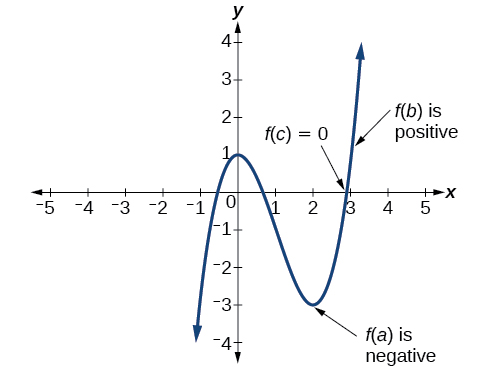$Graph of an odd-degree polynomial function that shows a point f(a) that’s negative, f(b) that’s positive, and f(c) that’s 0.$ The Intermediate Value Theorem states that for two numbers $a$ and $b$ in the domain of $f$, if $a<b$ and $f(a){\neq}f(b)$, then the function $f$ takes on every value between $f(a)$ and $f(b)$. We can apply this theorem to a special case that is useful in graphing polynomial functions. If a point on the graph of a continuous function $f$ at $x=a$ lies above the x-axis and another point at $x=b$ lies below the $x$-axis, there must exist a third point between $x=a$ and $x=b$ where the graph crosses the $x$-axis. Call this point $(c,f(c))$. This means that we are assured there is a solution $c$ where $f(c)=0$.

In other words, the Intermediate Value Theorem tells us that when a polynomial function changes from a negative value to a positive value (or vice versa), the function must cross the $x$-axis. The figure on the right shows that there is a zero between $a$ and $b$.

Intermediate Value Theorem

Let $f$ be a polynomial function. The Intermediate Value Theorem states that if $f(a)$ and $f(b)$ have opposite signs, then there exists at least one value $c$ between $a$ and $b$ for which $f(c)=0$.

Example $\PageIndex{7}$: Use the Intermediate Value Theorem

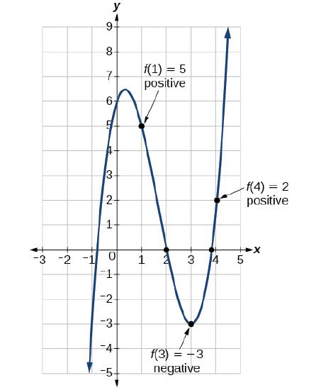
Show that the function $f(x)=x^3−5x^2+3x+6$ has at least two real zeros between $x=1$ and $x=4$.

Solution

As a start, evaluate $f(x)$ at the integer values $x=1,\;2,\;3,\; \text{and }4$.


$x$	1	2	3	4
$f(x)$	5	0	-3	2

One zero occurs at $x=2$. Also, since $f(3)$ is negative and $f(4)$ is positive, by the Intermediate Value Theorem, there must be at least one real zero between 3 and 4. Therefore, there are at least two real zeros between $x=1$ and $x=4$.

Analysis

We can also see on the graph of the function in Figure $\PageIndex{19}$ that there are two real zeros between $x=1$ and $x=4$.

$Graph of f(x)=x^3-5x^2+3x+6 and shows, by the Intermediate Value Theorem, that there exists two zeros since f(1)=5 and f(4)=2 are positive and f(3) = -3 is negative.$

Figure $\PageIndex{19}$

$try-it.png$ Try It $\PageIndex{7}$

Show that the function $f(x)=7x^5−9x^4−x^2$ has at least one real zero between $x=1$ and $x=2$.

Answer: Because $f$ is a polynomial function and since $f(1)$ is negative and $f(2)$ is positive, there is at least one real zero between $x=1$ and $x=2$.

The following example describes how using these two theorems can be incorporated into a search for zeros.

Example $\PageIndex{8}$: FInd all the zeros of a 4th degree polynomial

Let $f(x) = 2x^4+4x^3-x^2-6x-3$.

Solution

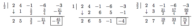
1. Possible rational zeros are $\pm \, 1$, $\pm \, 3$, $\pm \, \frac{1}{2}$, and $\pm \, \frac{3}{2}$.

Try our positive rational zeros, starting with the smallest, $\frac{1}{2}$. Since the remainder isn't zero, $\frac{1}{2}$ isn't a zero. Sadly, the final line in the division tableau has both positive and negative numbers, so $\frac{1}{2}$ is not an upper bound. The only information we get from this division is courtesy of the Remainder Theorem which tells us $f\left(\frac{1}{2}\right) = -\frac{45}{8}$ so the point $\left(\frac{1}{2}, -\frac{45}{8}\right)$ is on the graph of $f$.

Continue to our next possible zero, $1$. As before, the only information we can glean from this is that $(1,-4)$ is on the graph of $f$. When we try our next possible zero, $\frac{3}{2}$, we get that it is not a zero. We also see that it is an upper bound on the zeros of $f$, since all of the numbers in the final line of the division tableau are positive. This means there is no point trying our last possible rational zero, $3$.

The Intermediate Value Theorem indicates there is a zero between $1$ and $\frac{3}{2}$, since $f(1) < 0$ and $f\left(\frac{3}{2}\right) > 0$. Since there is no number in the list of rational zeros between $1$ and $\frac{3}{2}$, the zero must be an irrational number.

$3.3.6a.png$

Examine negative real zeros. Try the largest possible zero, $-\frac{1}{2}$. Synthetic division shows it is not a zero, nor is it a lower bound (since the numbers in the final line of the division tableau do not alternate), so we proceed to $-1$. This division shows $-1$ is a zero. Try $-1$ again, and it works once more. At this point, we have taken $f$, a fourth degree polynomial, and performed two successful divisions. Our quotient polynomial is quadratic, so look at it to find the remaining zeros.

$3.3.6b.png$

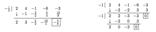
Setting the quotient polynomial equal to zero yields $2x^2 - 3 = 0$, so that $x^2 = \frac{3}{2}$, or $x = \pm \, \frac{\sqrt{6}}{2}$.

$3.3.2.png$ Thus $-1$ is a zero of multiplicity $2$ and zeros $\pm \frac{\sqrt{6}}{2}$ both have multiplicity $1$.

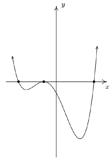
We know the end behavior of $y=f(x)$ resembles that of its leading term $y=2x^4$. This means that the graph enters the scene in Quadrant II and exits in Quadrant I. Since $\pm \, \frac{\sqrt{6}}{2}$ are zeros of odd multiplicity, we have that the graph crosses through the $x$-axis at the points $\left( -\frac{\sqrt{6}}{2}, 0 \right)$ and $\left( \frac{\sqrt{6}}{2}, 0 \right)$. Since $-1$ is a zero of multiplicity $2$, the graph of $y=f(x)$ touches and rebounds off the $x$-axis at $(-1,0)$. Putting this together, we get the sketch in the figure to the right.

Descartes’ Rule of Signs

There is a straightforward way to determine the possible numbers of positive and negative real zeros for any polynomial function. If the polynomial is written in descending order, Descartes’ Rule of Signs tells us of a relationship between the number of sign changes in $f(x)$ and the number of positive real zeros. For example, the polynomial function below has one sign change.

$CNX_Precalc_Figure_03_06_003.jpg$

This tells us that the function must have 1 positive real zero.

There is a similar relationship between the number of sign changes in $f(−x)$ and the number of negative real zeros.

$CNX_Precalc_Figure_03_06_004.jpg$

In this case, $f(−x)$ has 3 sign changes. This tells us that $f(x)$ could have 3 or 1 negative real zeros.

DESCARTES’ RULE OF SIGNS

According to Descartes’ Rule of Signs, if we let $f(x)=a_nx^n+a_{n−1}x^{n−1}+...+a_1x+a_0$ be a polynomial function with real coefficients:

The number of positive real zeros is either equal to the number of sign changes of $f(x)$ or is less than the number of sign changes by an even integer.
The number of negative real zeros is either equal to the number of sign changes of $f(−x)$ or is less than the number of sign changes by an even integer.

Example $\PageIndex{9}$: Use Descartes’ Rule of Signs

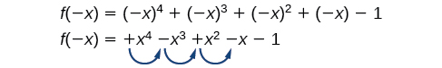
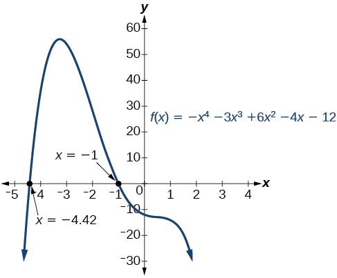
Use Descartes’ Rule of Signs to determine the possible numbers of positive and negative real zeros for $f(x)=−x^4−3x^3+6x^2−4x−12$.

Solution:

Begin by determining the number of sign changes.

$The function, f(x)=-x^4-3x^3+6x^2-4x-12, has two sign change between -3x^3 and 6x^2, and 6x^2 and -4x.`$

There are two sign changes, so there are either 2 or 0 positive real roots. Next, we examine $f(−x)$ to determine the number of negative real roots.

\[ \begin{align*} f(−x) & =−{(−x)}^4−3{(−x)}^3+6{(−x)}^2−4(−x)−12 \\ f(−x) & =−x^4+3x^3+6x^2+4x−12 \end{align*} \]

$The function, f(-x)=-x^4+3x^3+6x^2+4x-12, has two sign change between -x^4 and 3x^3, and 4x and -12.`$

Again, there are two sign changes, so there are either 2 or 0 negative real roots. There are four possibilities, as we can see in Table $\PageIndex{9}$.

Table $\PageIndex{9}$
Positive Real Zeros	Negative Real Zeros	Complex Zeros	Total Zeros
2	2	0	4
2	0	2	4
0	2	2	4
0	0	4	4

Analysis We can confirm the numbers of positive and negative real roots by examining a graph of the function. See Figure $\PageIndex{9}$. We can see from the graph that the function has 0 positive real roots and 2 negative real roots.

$Graph of f(x)=-x^4-3x^3+6x^2-4x-12 with x-intercepts at -4.42 and -1.$

Figure $\PageIndex{9}$.

$try-it.png$ Try It $\PageIndex{9}$

Use Descartes’ Rule of Signs to determine the maximum possible numbers of positive and negative real zeros for $f(x)=2x^4−10x^3+11x^2−15x+12$. Use a graph to verify the numbers of positive and negative real zeros for the function.

Answer: There must be 4, 2, or 0 positive real roots and 0 negative real roots. The graph shows that there are 2 positive real zeros and 0 negative real zeros.

Use the Fundamental Theorem of Algebra to find an interval where a zero exists

Now that we can find rational zeros for a polynomial function, we will look at a theorem that discusses the number of complex zeros of a polynomial function. The Fundamental Theorem of Algebra tells us that every polynomial function has at least one complex zero. This theorem forms the foundation for solving polynomial equations.

Suppose $f$ is a polynomial function of degree four, and $f (x)=0$. The Fundamental Theorem of Algebra states that there is at least one complex solution, call it $c_1$. By the Factor Theorem, we can write $f(x)$ as a product of $x−c_1$ and a polynomial quotient. Since $x−c_1$ is linear, the polynomial quotient will be of degree three. Now we apply the Fundamental Theorem of Algebra to the third-degree polynomial quotient. It will have at least one complex zero, call it $c_2$. So we can write the polynomial quotient as a product of $x−c_2$ and a new polynomial quotient of degree two. Continue to apply the Fundamental Theorem of Algebra until all of the zeros are found. There will be four of them and each one will yield a factor of $f(x)$.

THE FUNDAMENTAL THEOREM OF ALGEBRA

The Fundamental Theorem of Algebra states that, if $f(x)$ is a polynomial of degree $n > 0$, then $f(x)$ has at least one complex zero. We can use this theorem to argue that, if $f(x)$ is a polynomial of degree $n >0$, and a is a non-zero real number, then $f(x)$ has exactly $n$ linear factors

\[f(x)=a(x−c_1)(x−c_2)...(x−c_n) \nonumber\]

where $c_1, \;c_2$,..., $c_n$ are complex numbers. Therefore, $f(x)$ has $n$ roots if we allow for multiplicities.

$QA.png$ Does every polynomial have at least one imaginary zero?

No. Real numbers are a subset of complex numbers, but not the other way around. A complex number is not necessarily imaginary. Real numbers are also complex numbers.

Example $\PageIndex{10}$: Find the Zeros of a Polynomial Function with Complex Zeros

Find the zeros of $f(x)=3x^3+9x^2+x+3$.

Solution:

The Rational Zero Theorem tells us that if $\dfrac{p}{q}$ is a zero of $f(x)$, then $p$ is a factor of 3 and $q$ is a factor of 3.

\[ \begin{align*} \dfrac{p}{q}=\dfrac{\text{factor of constant term}}{\text{factor of coefficient}} &=\dfrac{\text{factor of }3}{\text{factor of }3} \end{align*}\]

The factors of 3 are ±1 and ±3. The possible values for $\dfrac{p}{q}$, and therefore the possible rational zeros for the function, are ±3, ±1, and $±\tfrac{1}{3}$. We will use synthetic division to evaluate each possible zero until we find one that gives a remainder of 0. Let’s begin with –3.

$xCNX_CAT_Figure_05_01_013.jpg$

The remainder is 0, so –3 is a zero of the function and the polynomial can be written as $(x+3)(3x^2+1) $

The other zeros can be found by setting the quadratic equal to 0 and solving for $x$.

$ 3x^2+1=0 \quad\longrightarrow\quad x^2 =−\dfrac{1}{3} \quad\longrightarrow\quad x=±\sqrt{−\dfrac{1}{3}} \quad\longrightarrow\quad x=±\dfrac{i\sqrt{3}}{3}$

Analysis

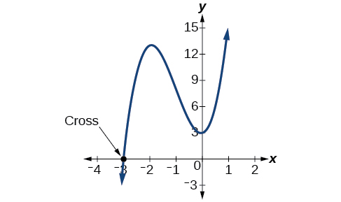$CNX_Precalc_Figure_03_06_002.jpg$ Look at the graph of the function $f$ in the figure to the right. Notice that, at $x =−3$, the graph crosses the $x$ axis, indicating an odd multiplicity (1) for the zero $x=–3$. Also note the presence of the two turning points. This means that, since there is a $3^{rd}$ degree polynomial, we are looking at the maximum number of turning points. So, the end behavior of increasing without bound to the right and decreasing without bound to the left will continue. Thus, all the $x$-intercepts for the function are shown. So either the multiplicity of $x=−3$ is 1 and there are two complex solutions, which is what we found, or the multiplicity at $x =−3$ is three. Either way, our result is correct.

$try-it.png$ Try It $\PageIndex{10}$

Find the zeros of $f(x)=2x^3+5x^2−11x+4$.

Answer: The zeros are $–4$, $\frac{1}{2}$, and $1$

Use the Linear Factorization Theorem to Find Polynomials with Given Zeros

A vital implication of the Fundamental Theorem of Algebra, as we stated above, is that a polynomial function of degree $n$ will have $n$ zeros in the set of complex numbers, if we allow for multiplicities. This means that we can factor the polynomial function into $n$ factors.

The Linear Factorization Theorem

The Linear Factorization Theorem states that a polynomial function will have the same number of factors as its degree, and that each factor will be in the form $(x−c)$, where $c$ is a complex number.

Let $f$ be a polynomial function with real coefficients, and suppose $a +bi$, $b≠0$, is a zero of $f(x)$. Then, by the Factor Theorem, $x−(a+bi)$ is a factor of $f(x)$. For $f$ to have real coefficients, $x−(a−bi)$ must also be a factor of $f(x)$. This is true because any factor other than $x−(a−bi)$, when multiplied by $x−(a+bi)$, will leave imaginary components in the product. Only multiplication with conjugate pairs will eliminate the imaginary parts and result in real coefficients. In other words, if a polynomial function $f$ with real coefficients has a complex zero $a +bi$, then the complex conjugate $a−bi$ must also be a zero of $f(x)$. This is called the Complex Conjugate Theorem.

COMPLEX CONJUGATE THEOREM

If the polynomial function $f$ has real coefficients and a complex zero in the form $a+bi$, then the complex conjugate of the zero, $a−bi$, is also a zero.

If the polynomial function $f$ has rational coefficients and a zero in the form $a+c\sqrt{b}$, and $b$ is not a perfect square, then the conjugate $a-c\sqrt{b}$, is also a zero.

$how-to.png$ How to: Construct a polynomial function given its zeroes.

Use the zeros to construct the linear factors of a general polynomial, $y=p(x)$.
To find the specific polynomial, $y=a \cdot p(x)$ that goes through point $(c,f(c))$, substitute $(c,f(c))$ into the function to determine the value of $a$.
Multiply out the result and simplify.

Example $\PageIndex{11}$: Use the Linear Factorization Theorem to Find a Polynomial with Given Zeros

Find a fourth degree polynomial with real coefficients that has zeros of $–3$, $2$, $i$, such that $f(−2)=100$.

Solution:

Because $x =i$ is a zero, by the Complex Conjugate Theorem $x =–i$ is also a zero. The polynomial must have factors of $(x+3),(x−2),(x−i)$, and $(x+i)$. So the lowest degree polynomial with these four zeros is $ f(x) =(x+3)(x−2)(x−i)(x+i) $.

Now we are looking for a specific polynomial for which $f(−2)=100$. Substitute $x=–2$ and $f (-2)=100$ into $f (x)= a(x+3)(x−2)(x−i)(x+i)$ and solve for $a$.

\[\begin{align*} 100=a(-2+3)(-2-2)(-2-i)(-2+i) \\ 100=a(1)(-4)(4-i^2) \\ 100=a(-4)(4+1) \\ 100=a(−20) \\ −5=a \nonumber \end{align*} \]

So the polynomial function is $f(x)=−5(x^4+x^3−5x^2+x−6) $ or $ f(x)=−5x^4−5x^3+25x^2−5x+30 $

Analysis. We found that both $i$ and $−i$ were zeros, but only one of these zeros needed to be given. If $i$ is a zero of a polynomial with real coefficients, then $−i$ must also be a zero of the polynomial because $−i$ is the complex conjugate of $i$ .

$QA.png$ If $2+3i$ is a zero of a polynomial with real coefficients, would $2−3i$ also need to be a zero?

Yes. When any complex number with an imaginary component is given as a zero of a polynomial with real coefficients, the conjugate must also be a zero of the polynomial.

$try-it.png$ $\PageIndex{11}$

Find a third degree polynomial with real coefficients that has zeros of $5$ and $−2i$ such that $f (1)=10$.

Answer: $f(x)=−\frac{1}{2}x^3+\frac{5}{2}x^2−2x+10$

Key Concepts

To find $f(k)$, determine the remainder of the polynomial $f(x)$ when it is divided by $x−k$. This is known as the Remainder Theorem.
According to the Factor Theorem, $k$ is a zero of $f(x)$ if and only if $(x−k)$ is a factor of $f(x)$.
According to the Rational Zero Theorem, each rational zero of a polynomial function with integer coefficients will be equal to a factor of the constant term divided by a factor of the leading coefficient.
When the leading coefficient is 1, the possible rational zeros are the factors of the constant term.
Synthetic division can be used to find the zeros of a polynomial function.
According to the Fundamental Theorem, every polynomial function with degree greater than 0 has at least one complex zero.
Allowing for multiplicities, a polynomial function will have the same number of factors as its degree. Each factor will be in the form $(x−c)$, where $c$ is a complex number.
The number of positive real zeros of a polynomial function is either the number of sign changes of the function or less than the number of sign changes by an even integer.
The number of negative real zeros of a polynomial function is either the number of sign changes of $f(−x)$ or less than the number of sign changes by an even integer.

Glossary

Descartes’ Rule of Signs

a rule that determines the maximum possible numbers of positive and negative real zeros based on the number of sign changes of $f(x)$ and $f(−x)$

Factor Theorem

$k$ is a zero of polynomial function $f(x)$ if and only if $(x−k)$ is a factor of $f(x)$

Fundamental Theorem of Algebra

a polynomial function with degree greater than 0 has at least one complex zero

Intermediate Value Theorem

If two points of a polynomial are on opposite sides of the $x$-axis, there is at least one zero between them.

Linear Factorization Theorem

allowing for multiplicities, a polynomial function will have the same number of factors as its degree, and each factor will be in the form $(x−c)$, where $c$ is a complex number

Rational Zero Theorem

the possible rational zeros of a polynomial function have the form $\frac{p}{q}$ where $p$ is a factor of the constant term and $q$ is a factor of the leading coefficient.

Remainder Theorem

if a polynomial $f(x)$ is divided by $(x−k)$, then the remainder is equal to the value $f(k)$