3.7: The Reciprocal Function

Last updated
Save as PDF

Page ID: 44350

$ \newcommand{\vecs}[1]{\overset { \scriptstyle \rightharpoonup} {\mathbf{#1}} } $ $ \newcommand{\vecd}[1]{\overset{-\!-\!\rightharpoonup}{\vphantom{a}\smash {#1}}} $$\newcommand{\id}{\mathrm{id}}$ $ \newcommand{\Span}{\mathrm{span}}$ $ \newcommand{\kernel}{\mathrm{null}\,}$ $ \newcommand{\range}{\mathrm{range}\,}$ $ \newcommand{\RealPart}{\mathrm{Re}}$ $ \newcommand{\ImaginaryPart}{\mathrm{Im}}$ $ \newcommand{\Argument}{\mathrm{Arg}}$ $ \newcommand{\norm}[1]{\| #1 \|}$ $ \newcommand{\inner}[2]{\langle #1, #2 \rangle}$ $ \newcommand{\Span}{\mathrm{span}}$ $\newcommand{\id}{\mathrm{id}}$ $ \newcommand{\Span}{\mathrm{span}}$ $ \newcommand{\kernel}{\mathrm{null}\,}$ $ \newcommand{\range}{\mathrm{range}\,}$ $ \newcommand{\RealPart}{\mathrm{Re}}$ $ \newcommand{\ImaginaryPart}{\mathrm{Im}}$ $ \newcommand{\Argument}{\mathrm{Arg}}$ $ \newcommand{\norm}[1]{\| #1 \|}$ $ \newcommand{\inner}[2]{\langle #1, #2 \rangle}$ $ \newcommand{\Span}{\mathrm{span}}$$\newcommand{\AA}{\unicode[.8,0]{x212B}}$

Learning Objectives

Use arrow notation to describe asymptotic behaviour.
Use transformations to graph rational functions

Using Arrow Notation

We have seen the graphs of the basic reciprocal function and the squared reciprocal function from our study of toolkit functions. Examine these graphs, as shown in Figure $\PageIndex{1}$, and notice some of their features.

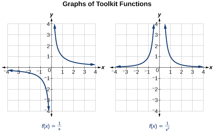
Graphs of f(x)=1/x and f(x)=1/x^2 — Figure $\PageIndex{1}$

Several things are apparent if we examine the graph of $f(x)=\dfrac{1}{x}$.

On the left branch of the graph, the curve approaches the $x$-axis $(y=0)$ as $x\rightarrow -\infty$.
As the graph approaches $x = 0$ from the left, the curve drops, but as we approach zero from the right, the curve rises.
Finally, on the right branch of the graph, the curves approaches the $x$-axis $(y=0) $ as $x\rightarrow \infty$.

To summarize, we use arrow notation to show that $x$ or $f (x)$ is approaching a particular value in the table below.

Symbol $\qquad$ Meaning

$ \begin{array}{ll}
x\rightarrow a^- & x \text{ approaches a from the left } x<a \text{ but close to } a\\
x\rightarrow a^+ & x \text{ approaches a from the right } x>a \text{ but close to } a\\
x\rightarrow \infty & x\text{ approaches infinity}\\
& \text{("increases without bound") }\\
x\rightarrow −\infty & x\text{ approaches negative infinity} \\
& \text{("decreases without bound") }\\
\end{array} $

Symbol $\qquad$ Meaning
$ \begin{array}{ll} f(x)\rightarrow \infty & \text{the output approaches infinity} \\ & \text{("increases without bound") } \\ f(x)\rightarrow −\infty & \text{ the output approaches negative infinity} \\ & \text{("decreases without bound") } \\ f(x)\rightarrow a & \text{ the output approaches } a\\ \end{array} $

$Graph of f(x)=1/x which highlights the segments of the turning points to denote their end behavior.$

Figure $\PageIndex{2}$. Illustration of arrow notation used for
$\color{Orange}{\text{Vertical Asymptote \(x=0$}}\) and
$\color{Cerulean}{\text{Horizontal Asymptote \(y=0$}}\)

Local Behavior of $f(x)=\frac{1}{x}$

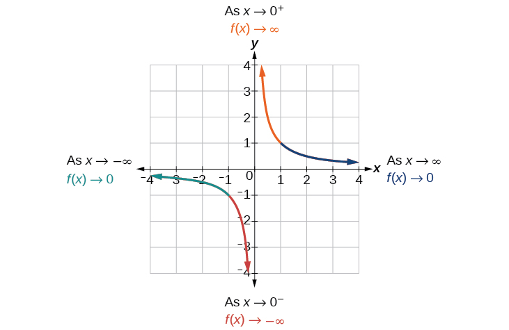
Let’s begin by looking at the reciprocal function, $f(x)=\frac{1}{x}$. We cannot divide by zero, which means the function is undefined at $x=0$; so zero is not in the domain. As the input values approach zero from the left side (becoming very small, negative values), the function values decrease without bound (in other words, they approach negative infinity).

Table $\PageIndex{1}$: Illustration of arrow notation - As $x\rightarrow 0^−,f(x)\rightarrow −\infty$
$x$	–0.1	–0.01	–0.001	–0.0001
$f(x)=\frac{1}{x}$	–10	–100	–1000	–10,000

As the input values approach zero from the right side (becoming very small, positive values), the function values increase without bound (approaching infinity).

Table $\PageIndex{2}$: Illustration of arrow notation - As $x\rightarrow 0^+, f(x)\rightarrow \infty$.
$x$	0.1	0.01	0.001	0.0001
$f(x)=\frac{1}{x}$	10	100	1000	10,000

See Figure $\PageIndex{3}$ for how this behaviour appears on a graph.

Definition: VERTICAL ASYMPTOTE

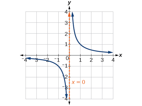$Graph of f(x)=1/x with its vertical asymptote at x=0.$ A vertical asymptote of a graph is a vertical line $x=a$ where the graph tends toward positive or negative infinity as the inputs approach $a$.

In arrow notation this is written

As $x\rightarrow a$, $f(x)\rightarrow \infty$, or as $x\rightarrow a$, $f(x)\rightarrow −\infty$.

This can also be written in limit notation as:

$ \displaystyle \lim_{x \to a}f(x) \rightarrow \infty$, or as $ \displaystyle \lim_{x \to a}f(x) \rightarrow -\infty$

Figure $\PageIndex{3}$: Example of a Vertical Asymptote, $x=0$

End Behavior of $f(x)=\frac{1}{x}$

As the values of $x$ approach infinity, the function values approach $0$. As the values of $x$ approach negative infinity, the function values approach $0$. See Figure $\PageIndex{4}$) for how this behaviour appears on a graph.. Symbolically, using arrow notation

As $x\rightarrow \infty$, $f(x)\rightarrow 0$, and as $x\rightarrow −\infty$, $f(x)\rightarrow 0$.

Based on this overall behavior and the graph, we can see that the function approaches 0 but never actually reaches 0; it seems to level off as the inputs become large. This behavior creates a horizontal asymptote, a horizontal line that the graph approaches as the input increases or decreases without bound. In this case, the graph is approaching the horizontal line $y=0$.

Definition: HORIZONTAL ASYMPTOTE

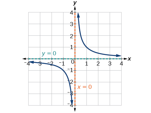$Graph of f(x)=1/x with its vertical asymptote at x=0 and its horizontal asymptote at y=0.$ A horizontal asymptote of a graph is a horizontal line $y=b$ where the graph approaches the line as the inputs increase or decrease without bound.

In arrow notation this is written

As $x\rightarrow \infty,$ $f(x)\rightarrow b$ or $ x\rightarrow −\infty$, $f(x)\rightarrow b$.

This can also be written in limit notation as:

$ \displaystyle \lim_{x \to \infty}f(x) \rightarrow b$, or $ \displaystyle \lim_{x \to -\infty}f(x) \rightarrow b$

Figure $\PageIndex{4}$: Example of a Horizontal Asymptote, $y=0$

Example $\PageIndex{1}$: Using Arrow Notation.

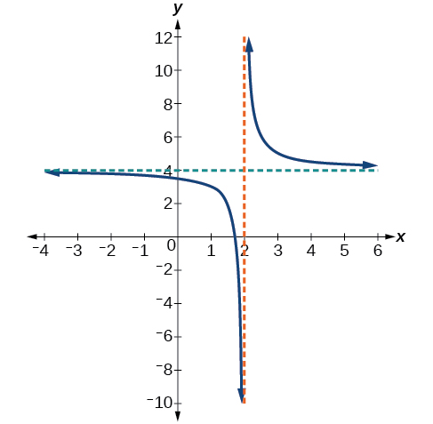
Use arrow notation to describe the end behavior and local behavior of the function graphed in below.

Graph of f(x)=1/(x-2)+4 with its vertical asymptote at x=2 and its horizontal asymptote at y=4.

Solution

Local Behaviour. Notice that the graph is showing a vertical asymptote at $x=2$, which tells us that the function is undefined at $x=2$.

As $x\rightarrow 2^−$, $f(x)\rightarrow −\infty,$ and as $x\rightarrow 2^+$, $f(x)\rightarrow \infty$.

End behaviour. And as the inputs decrease without bound, the graph appears to be leveling off at output values of $4$, indicating a horizontal asymptote at $y=4$. As the inputs increase without bound, the graph levels off at $4$.

As $x\rightarrow \infty$, $f(x)\rightarrow 4$ and as $x\rightarrow −\infty$, $f(x)\rightarrow 4$.

$try-it.png$ Try It $\PageIndex{1}$

Use arrow notation to describe the end behavior and local behavior for the reciprocal squared function.

Answer

End behavior: as $x\rightarrow \pm \infty$, $f(x)\rightarrow 0$;

Local behavior: as $x\rightarrow 0$, $f(x)\rightarrow \infty$ (there are no x- or y-intercepts)

Graphing using Transformations

When graphing vertical and horizontal shifts of the reciprocal function, the order in which horizontal and vertical translations are applied does not affect the final graph.

Example $\PageIndex{2}$:

Sketch the graph of $g ( x ) = \dfrac { 1 } { x - 5 } + 3$.

Solution

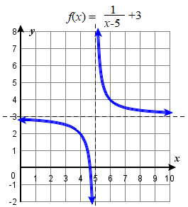$3.7 ex2.png graph of reciprocal function shifted right 5 and up 3$ Begin with the reciprocal function and identify the translations.

$\begin{array} { cl }
{ y = \dfrac{1}{x} } &\color{Cerulean}{Basic \:function} \\
{ y = \dfrac{1}{x-5} }&\color{Cerulean}{Horizontal \:shift \: right \:5 \:units} \\
{ y = \dfrac{1}{x-5} +3 } &\color{Cerulean}{Vertical \:shift \:up\:3 \:units}
\end{array}$

Start the graph by first drawing the vertical and horizontal asymptotes. Then use the location of the asymptotes to sketch in the rest of the graph.

It is easiest to graph translations of the reciprocal function by writing the equation in the form $y = \pm \dfrac{1}{x+c} +d$.

Example $\PageIndex{3}$:

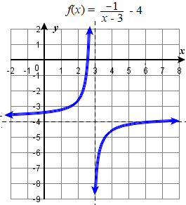
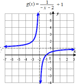
Sketch the graphs of $f(x) = \dfrac{-1}{x-3} - 4$ and $g(x) = \dfrac{1}{-x-2} +1$.

Solution

$\begin{array} { rl }
f(x) &= \dfrac{-1}{x-3} - 4\\
&= -\dfrac{1}{x-3}
\end{array}$

$\qquad\qquad$To graph $f$, start with the parent function $ y = \dfrac{1}{x,}$
$\qquad\qquad$shift right $3$ units, reflect over the $x$-axis,
$\qquad\qquad$and shift down $4$ units.

$3.7 #3a.png$

$\begin{array} { rl }
g(x) &= \dfrac{1}{-x-2} +1\\
&=\dfrac{1}{-(x+2)} +1 \\
&=- \dfrac{1}{x+2} +1
\end{array}$

$\qquad\qquad$To graph $g$, start with the parent function $ y = \dfrac{1}{x,}$
$\qquad\qquad$shift left $2$ units, reflect over the $x$-axis,
$\qquad\qquad$and shift up $1$ unit.

$3.7 #3b.png$

When a rational function consists of a linear numerator and linear denominator, it is actually just a translation of the reciprocal function. To see how to graph the function using transformations, long division or synthetic division on the original function must be done to obtain a more user friendly form of the equation.

Example $\PageIndex{4}$: Use Transformations to Graph a Rational Function.

Sketch a graph of the function $f(x)=\dfrac{3x+7}{x+2}.$ Identify the horizontal and vertical asymptotes of the graph, if any.

Solution

Use long division or synthetic division to obtain an equivalent form of the function, $f(x)=\dfrac{1}{x+2}+3$.

Written in this form, it is clear the graph is that of the reciprocal function shifted two units left and three units up.

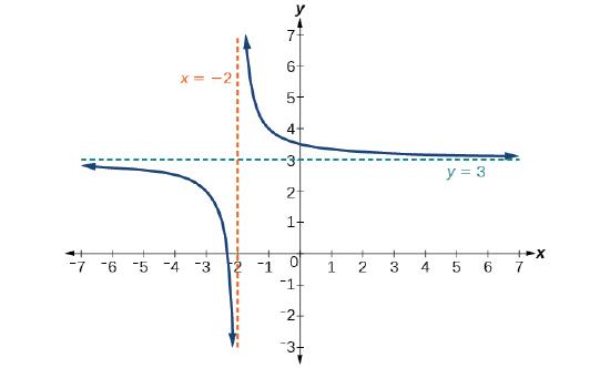$Graph of f(x)=1/(x+2)+3 with its vertical asymptote at x=-2 and its horizontal asymptote at y=3.$ The graph of the shifted function is displayed to the right.

Local Behaviour. Notice that this function is undefined at $x=−2$, and the graph also is showing a vertical asymptote at $x=−2$.

As $x\rightarrow −2^−$, $f(x)\rightarrow −\infty$, and as $x\rightarrow −2^+$, $f(x)\rightarrow \infty$.

End Behaviour. As the inputs increase and decrease without bound, the graph appears to be leveling off at output values of 3, indicating a horizontal asymptote at $y=3$.

As $x\rightarrow \pm \infty$, $f(x)\rightarrow 3$.

Analysis. Notice that horizontal and vertical asymptotes are shifted left 2 and up 3 along with the function.

$try-it.png$ Try It $\PageIndex{5}$: Graph and construct an equation from a description

State the transformations to perform on the graph of $y=\dfrac{1}{x}$ needed to graph $f(x) = \dfrac{18-14x}{x+32}$.

Answer: $f(x)=-\dfrac{1}{x+32}+14$. Shift left $32$ units, reflect over the $x$-axis, and shift up $14$ units.

$try-it.png$ Try It $\PageIndex{6}$: Graph and construct an equation from a description

Construct the equation, sketch the graph, and find the horizontal and vertical asymptotes of the reciprocal squared function that has been shifted right 3 units and down 4 units.

Answer

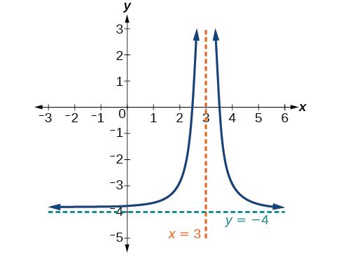$Graph of f(x)=1/(x-3)^2-4 with its vertical asymptote at x=3 and its horizontal asymptote at y=-4.$ The function and the asymptotes are shifted 3 units right and 4 units down.

As $x\rightarrow 3$, $f(x)\rightarrow \infty$, and as $x\rightarrow \pm \infty$, $f(x)\rightarrow −4$.

The function is $f(x)=\dfrac{1}{{(x−3)}^2}−4$.

Add texts here. Do not delete this text first.

\(x\)	–0.1	–0.01	–0.001	–0.0001
\(f(x)=\frac{1}{x}\)	–10	–100	–1000	–10,000

Using Arrow Notation

Local Behavior of \(f(x)=\frac{1}{x}\)

End Behavior of \(f(x)=\frac{1}{x}\)

Graphing using Transformations